Retarded Fields

We have found the solution to Maxwell's equations in terms of retarded potentials. Let us now construct the associated retarded electric and magnetic fields using (see Section 1.3)

$${\bf E} = - \nabla\phi - \frac{\partial {\bf A}}{\partial t},$$ (77)

$${\bf B} = \nabla\times{\bf A}.$$ (78)

It is helpful to write

$${\bf R} = {\bf r} - {\bf r}',$$ (79)

where $R=\vert{\bf r}-{\bf r}'\vert$ . The retarded time becomes $t_r = t- R/c$ , and a general retarded quantity is written $[F({\bf r}', t)]\equiv F({\bf r}', t_r)$ . Thus, we can express the retarded potential solutions of Maxwell's equations in the particularly compact form

$$\phi({\bf r},t) = \frac{1}{4\pi\, \epsilon_0} \int \frac{[\rho]}{R} \,dV',$$ (80)

$${\bf A}({\bf r}, t) = \frac{\mu_0}{4\pi} \int \frac{[{\bf j}]}{R} \,dV'.$$ (81)

It is easily seen that

$$\nabla\phi = \frac{1}{4\pi\,\epsilon_0}\int \left( [\rho]\, \nabla\left(R^{\,-1}\right) + \frac{[\partial\rho/\partial t]}{R}\, \nabla t_r\right)dV'$$

$$= - \frac{1}{4\pi\,\epsilon_0} \int \left( \frac{[\rho]}{R^{\,3}}\,{\bf R} + \frac{[\partial\rho/\partial t]}{c\,R^{\,2}}\,{\bf R} \right) \,dV',$$ (82)

where use has been made of

$$\nabla R = \frac{\bf R}{R},~~~\nabla\left( R^{\,-1}\right)= - \frac{\bf R}{R^{\,3}},~~~\nabla t_r = - \frac{\bf R}{c\,R}.$$ (83)

Likewise,

$$\nabla\times{\bf A} = \frac{\mu_0}{4\pi} \int \left( \nabla\left(R^{\,-1}\right) \times [{\bf j}] + \frac{\nabla t_r\times [\partial {\bf j}/\partial t]}{R} \right)dV'$$

$$= -\frac{\mu_0}{4\pi} \int \left( \frac{{\bf R} \times [{\bf j}]}... ...} + \frac{{\bf R} \times [\partial {\bf j}/\partial t]}{c\,R^{\,2}} \right)dV'.$$ (84)

Equations (77), (78), (82), and (84) can be combined to give

$${\bf E} = \frac{1}{4\pi\,\epsilon_0} \int \left( [\rho] \,\frac{\... ... R}{c\,R^{\,2}} - \frac{[\partial {\bf j}/\partial t]}{c^{\,2} \,R} \right)dV',$$ (85)

and

$${\bf B} = \frac{\mu_0}{4\pi} \int \left( \frac{ [{\bf j}]\times {... ...+ \frac{ [\partial {\bf j}/\partial t]\times {\bf R} } {c\,R^{\,2}} \right)dV'.$$ (86)

Suppose that our charges and currents vary on some characteristic timescale $t_0$ . Let us define $R_0 = c\, t_0$ , which is the distance a light ray travels in time $t_0$ . We can evaluate Equations (85) and (86) in two asymptotic regions: the near field region $R\ll R_0$ , and the far field region $R\gg R_0$ . In the near field region,

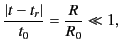$$\frac{\vert t -t_r\vert}{t_0} = \frac{R}{R_0} \ll 1,$$ (87)

so the difference between retarded time and standard time is relatively small. This allows us to expand retarded quantities in a Taylor series. Thus,

$$[\rho] \simeq \rho + \frac{\partial\rho}{\partial t} \,(t_r-t) + \frac{1}{2} \frac{\partial^{\,2} \rho}{\partial t^{\,2}}\,(t_r -t )^2+\cdots,$$ (88)

giving

$$[\rho] \simeq \rho - \frac{\partial \rho}{\partial t} \frac{R}{c}... ... \frac{\partial^{\,2} \rho}{\partial t^{\,2}} \frac{R^{\,2}}{c^{\,2}} + \cdots.$$ (89)

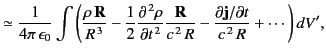
Expansion of the retarded quantities in the near field region yields

$${\bf E}({\bf r},t) \simeq \frac{1}{4\pi \,\epsilon_0} \int \left( \frac{\rho\,{\bf R... ...^{\,2}\, R} - \frac{\partial {\bf j}/\partial t}{c^{\,2} \,R}+\cdots\right)dV',$$ (90)

$${\bf B} ({\bf r},t) \simeq \frac{\mu_0}{4\pi} \int \left(\frac{{\bf j}\times{\bf R}}{... ...\,2} {\bf j}/ \partial t^{\,2})\times{\bf R}}{c^{\,2}\, R} +\cdots \right) dV'.$$ (91)

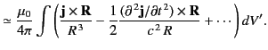
In Equation (90), the first term on the right-hand side corresponds to Coulomb's law, the second term is the lowest order correction to Coulomb's law due to retardation effects, and the third term corresponds to Faraday induction. In Equation (91), the first term on the right-hand side is the Biot-Savart law, and the second term is the lowest order correction to the Biot-Savart law due to retardation effects. Note that the retardation corrections are only of order $(R/R_0)^2$ . We might suppose, from looking at Equations (85) and (86), that the corrections should be of order $R/R_0$ . However, all of the order $R/R_0$ terms canceled out in the previous expansion.

In the far field region, $R\gg R_0$ , Equations (85) and (86) are dominated by the terms that vary like $R^{\,-1}$ , so that

$${\bf E}({\bf r},t) \simeq -\frac{1}{4\pi\,\epsilon_0}\int\frac{[\partial {\bf j}_\perp /\partial t]}{c^{\,2} \,R} \,dV',$$ (92)

$${\bf B} ({\bf r},t) \simeq \frac{\mu_0}{4\pi} \int \frac{ [\partial {\bf j}_\perp/\partial t]\times {\bf R} } {c\,R^{\,2}}\,dV',$$ (93)

where

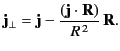$${\bf j}_\perp = {\bf j} - \frac{({\bf j} \cdot {\bf R})}{R^{\,2}}\, {\bf R}.$$ (94)

Here, use has been made of $[\partial \rho/\partial t] = -[\nabla\cdot {\bf j}]$ and $[\nabla\cdot {\bf j} ] \simeq -[\partial {\bf j}/\partial t]\cdot {\bf R}/(c \,R)$ . Suppose that our charges and currents are localized to some finite region of space in the vicinity of the origin, and that the extent of the current-and-charge-containing region is much less than $\vert{\bf r}\vert$ . It follows that retarded quantities can be written

$$[ \rho({\bf r}', t)] \simeq \rho({\bf r}', t - r/c),$$ (95)

et cetera. Thus, the electric field reduces to

$${\bf E}({\bf r},t) \simeq -\frac{1}{4\pi\,\epsilon_0} \frac{\left[ \int \partial {\bf j}_\perp/\partial t\,\,dV'\right]}{c^{\,2}\, r},$$ (96)

whereas the magnetic field is given by

$${\bf B}({\bf r},t) \simeq \frac{1}{4\pi\,\epsilon_0} \frac{ \left... ...ial {\bf j}_\perp /\partial t\,\,dV'\right] \times{\bf r} }{c^{\,3} \,r^{\,2}}.$$ (97)

Here, $[\cdots]$ merely denotes evaluation at the retarded time $t-r/c$ . Note that

$$\frac{E}{B} = c,$$ (98)

and

$${\bf E} \cdot {\bf B} = 0.$$ (99)

This configuration of electric and magnetic fields is characteristic of an electromagnetic wave. In fact, Equations (96) and (97) describe an electromagnetic wave propagating radially away from the charge and current containing region. The wave is clearly driven by time-varying electric currents. Now, charges moving with a constant velocity constitute a steady current, so a nonsteady current is associated with accelerating charges. We conclude that accelerating electric charges emit electromagnetic waves. The wave fields, (96) and (97), fall off like the inverse of the distance from the wave source. This behavior should be contrasted with that of Coulomb or Biot-Savart fields, which fall off like the inverse square of the distance from the source.

In conclusion, electric and magnetic fields look simple in the near field region (they are just Coulomb fields, etc.), and also in the far field region (they are just electromagnetic waves). Only in the intermediate region, $R\sim R_0$ , do the fields get really complicated.