Next: Exercises
Up: Resonant Cavities and Waveguides
Previous: Waveguides
We have seen that it is possible to propagate electromagnetic
waves down a hollow conductor. However, other types of guiding structures
are also possible. The general requirement for a guide of electromagnetic
waves is that there be a flow of energy along the axis of the guiding
structure, but not perpendicular to the axis. This implies that the electromagnetic
fields
are appreciable only in the immediate neighborhood of the guiding structure.
Consider a uniform cylinder of arbitrary
cross-section made of some dielectric material, and surrounded by a vacuum.
This structure can serve as a waveguide provided the dielectric
constant of the material is sufficiently large. Note, however, that
the boundary conditions satisfied by the electromagnetic fields
are significantly different to those of a conventional waveguide.
The transverse fields are governed by two equations: one for the
region inside the dielectric, and the other for the vacuum region.
Inside the dielectric, we have
![$\displaystyle \left[ \nabla_s^{\,2} +\left(\epsilon_1 \,\frac{\omega^{\,2}}{c^{\,2}} - k_g^{\,2}\right) \right]\psi = 0.$](img2906.png) |
(1372) |
In the vacuum region, we have
![$\displaystyle \left[ \nabla_s^{\,2} +\left( \frac{\omega^{\,2}}{c^{\,2}} - k_g^{\,2}\right) \right]\psi = 0.$](img2907.png) |
(1373) |
Here,
 stands for either
  or
or  ,
,
 is the relative
permittivity of the dielectric material, and
is the relative
permittivity of the dielectric material, and  is the guide propagation
constant. The propagation constant must be the same both inside and
outside the dielectric in order to allow the electromagnetic boundary
conditions to be satisfied at all points on the surface of the cylinder.
is the guide propagation
constant. The propagation constant must be the same both inside and
outside the dielectric in order to allow the electromagnetic boundary
conditions to be satisfied at all points on the surface of the cylinder.
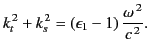
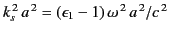
Inside the dielectric, the transverse Laplacian must be negative, so that the
constant
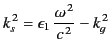 |
(1374) |
is positive. Outside the cylinder the requirement of no transverse flow
of energy can only be satisfied if the fields fall off exponentially
(instead of oscillating). Thus,
 |
(1375) |
must be positive.
The oscillatory solutions (inside) must be matched to the exponentiating
solutions (outside). The boundary conditions are the continuity
of normal  and
and  and tangential
  and
and  on the surface of the tube. These boundary conditions are far more complicated
than those in a conventional waveguide. For this reason, the normal
modes cannot usually be classified as either pure TE or pure TM modes.
In general, the normal modes possess both electric and magnetic field
components in the transverse plane. However, for the special case of a
dielectric cylinder tube of circular cross-section, the normal modes can
have either pure TE
or pure TM characteristics. Let us examine this case in detail.
on the surface of the tube. These boundary conditions are far more complicated
than those in a conventional waveguide. For this reason, the normal
modes cannot usually be classified as either pure TE or pure TM modes.
In general, the normal modes possess both electric and magnetic field
components in the transverse plane. However, for the special case of a
dielectric cylinder tube of circular cross-section, the normal modes can
have either pure TE
or pure TM characteristics. Let us examine this case in detail.
Consider a dielectric cylinder of dielectric constant
whose transverse cross-section is a circle of radius  . For the sake of simplicity, let us only search for normal
modes whose electromagnetic fields have no azimuthal variation.
Equations (1374) and (1376) yield
. For the sake of simplicity, let us only search for normal
modes whose electromagnetic fields have no azimuthal variation.
Equations (1374) and (1376) yield
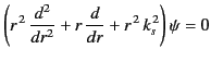 |
(1376) |
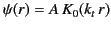
for  . The general solution to this equation is some linear combination
of the Bessel functions
. The general solution to this equation is some linear combination
of the Bessel functions
 and
and
 . However, because
is badly behaved at the origin (
. However, because
is badly behaved at the origin ( ), the physical solution
is
), the physical solution
is
 .
.
Equations (1375) and (1377) yield
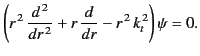 |
(1377) |
which can be rewritten
 |
(1378) |
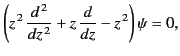
where  . The above can be recognized as a type of modified Bessel equation, whose
most general form is
. The above can be recognized as a type of modified Bessel equation, whose
most general form is
![$\displaystyle \left[z^{\,2}\,\frac{d^2}{d z^2} + z\,\frac{d}{dz} - (z^{\,2}+m^{\,2})\right] \psi = 0.$](img2918.png) |
(1379) |
The two linearly independent solutions of the previous equation are denoted
 and
and  .
Moreover,
.
Moreover,
 as
as
 , whereas
 .
Thus, it is clear that the physical solution to
Equation (1379) (i.e., the one that decays as
.
Thus, it is clear that the physical solution to
Equation (1379) (i.e., the one that decays as
 )
is
)
is
 .
.
The physical solution is then
 |
(1380) |
for  , and
, and
 |
(1381) |
for  . Here,
  is an arbitrary constant, and
 stands for
either
or
. It follows from Equations (1335)-(1336) (using
stands for
either
or
. It follows from Equations (1335)-(1336) (using
 ) that
 |
 |
(1382) |
 |
 |
(1383) |
 |
 |
(1384) |
 |
 |
(1385) |
for
. There are an analogous set of relations for
.
The fact that the field components form two groups--that is, ( ,
,  ),
which depend on
, and (
),
which depend on
, and ( ,
,  ), which depend
on
--implies that the normal modes
take the form of either pure TE modes or pure TM modes.
), which depend
on
--implies that the normal modes
take the form of either pure TE modes or pure TM modes.
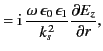
For a TE mode ( ) we find that
for
, and
for
. Here we have used the identities
where  denotes differentiation with respect to
  . The boundary conditions
require
. The boundary conditions
require  ,
,  , and
, and
 to be continuous across
  . Thus,
it follows that
. Thus,
it follows that
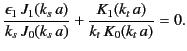
Eliminating the arbitrary constant
between the above two equations yields the dispersion relation
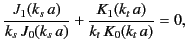 |
(1396) |
where
 |
(1397) |
Figure:
Graphical solution of the dispersion relation (1398). The curve
represents
 . The curve
  represents
 .
.
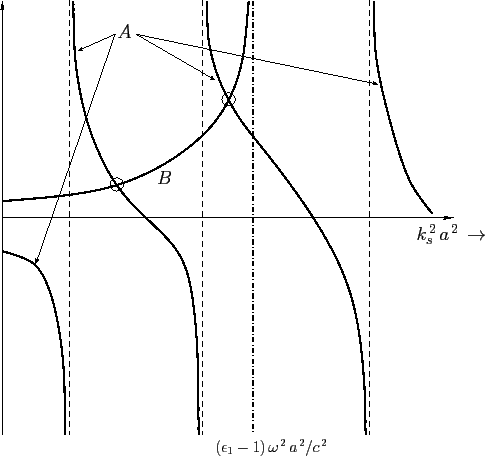 |
Figure 26 shows a graphical solution of the above dispersion relation.
The roots correspond to the crossing points of the two curves;
 and
.
The vertical asymptotes of the first curve are given by the roots
of
and
.
The vertical asymptotes of the first curve are given by the roots
of
 . The vertical asymptote of the second curve occurs
when
. The vertical asymptote of the second curve occurs
when  : that is, when
 .
Note, from Equation (1399), that
.
Note, from Equation (1399), that  decreases as
  increases. In Figure 26,
there are two crossing points, corresponding to two distinct propagating
modes of
the system. It is evident that if the point
corresponds to
a value of
increases. In Figure 26,
there are two crossing points, corresponding to two distinct propagating
modes of
the system. It is evident that if the point
corresponds to
a value of  that is less than the first root of
then there is no crossing of the two curves, and, hence, there
are no propagating modes. Because the first root
of
that is less than the first root of
then there is no crossing of the two curves, and, hence, there
are no propagating modes. Because the first root
of  occurs at
  (see Table 2), the condition for the
existence of propagating modes can be written
(see Table 2), the condition for the
existence of propagating modes can be written
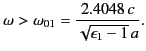 |
(1398) |
In other words, the mode frequency must lie above the cutoff frequency
 for
the
for
the
 mode [here, the 0 corresponds to the number
of nodes in the azimuthal direction, and the 1 refers to the first root
of
]. It is also evident that, as the mode frequency is
gradually increased, the point
eventually crosses the second
vertical asymptote of
, at which point the
mode [here, the 0 corresponds to the number
of nodes in the azimuthal direction, and the 1 refers to the first root
of
]. It is also evident that, as the mode frequency is
gradually increased, the point
eventually crosses the second
vertical asymptote of
, at which point the
 mode can propagate. As
  is further increased,
more and more TE modes can propagate. The cutoff frequency for
the
is further increased,
more and more TE modes can propagate. The cutoff frequency for
the
 mode is given by
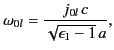 |
(1399) |
where  is
is  th root of
(in order of increasing
).
th root of
(in order of increasing
).
At the cutoff frequency for a particular mode,
, which implies from
Equation (1377) that
 . In other words, the mode propagates
along the guide at the velocity of light in vacuum. At frequencies below
this cutoff frequency, the system no longer acts as a guide, but rather as
an antenna, with energy being radiated radially. For frequencies
well above the cutoff,
and
are of the same order of magnitude,
and are large compared to
. This implies that the fields
do not extend appreciably outside the dielectric cylinder.
. In other words, the mode propagates
along the guide at the velocity of light in vacuum. At frequencies below
this cutoff frequency, the system no longer acts as a guide, but rather as
an antenna, with energy being radiated radially. For frequencies
well above the cutoff,
and
are of the same order of magnitude,
and are large compared to
. This implies that the fields
do not extend appreciably outside the dielectric cylinder.
For a TM mode ( ) we find that
for
, and
for
. The boundary conditions require  ,
,
 , and
, and
 to be continuous across
. Thus, it follows that
to be continuous across
. Thus, it follows that
Eliminating the arbitrary constant
between the above two equations yields the dispersion relation
 |
(1408) |
It is clear, from this dispersion relation,
that the cutoff frequency for the
 mode is
exactly the same as that for the
mode. It is also clear that,
in the limit
mode is
exactly the same as that for the
mode. It is also clear that,
in the limit
 , the propagation constants are determined
by the roots of
, the propagation constants are determined
by the roots of
 . However, this is
exactly the same as
the determining equation for TE modes in a metallic waveguide of circular cross-section
(filled with dielectric of relative permittivity
).
. However, this is
exactly the same as
the determining equation for TE modes in a metallic waveguide of circular cross-section
(filled with dielectric of relative permittivity
).
Modes with azimuthal dependence (i.e.,  ) have longitudinal components of both
and
. This makes the mathematics
somewhat more complicated. However, the basic results are the same as
for
) have longitudinal components of both
and
. This makes the mathematics
somewhat more complicated. However, the basic results are the same as
for  modes: that is, for frequencies well above the cutoff frequency the
modes are localized in the immediate vicinity of the cylinder.
modes: that is, for frequencies well above the cutoff frequency the
modes are localized in the immediate vicinity of the cylinder.
Next: Exercises
Up: Resonant Cavities and Waveguides
Previous: Waveguides
Richard Fitzpatrick
2014-06-27