Suppose that the direction of symmetry is along the ![]() -axis, and that
the length of the cavity in this direction is
-axis, and that
the length of the cavity in this direction is ![]() . The boundary
conditions at
. The boundary
conditions at ![]() and
and ![]() demand that the
demand that the ![]() dependence of wave
quantities be either
dependence of wave
quantities be either
![]() or
or
![]() ,
where
,
where
![]() . In other words,
all wave quantities satisfy
. In other words,
all wave quantities satisfy
| (1328) |
| (1329) | ||
| (1330) |
Let us write each vector and each operator in the above equations
as the sum of a transverse part, designated by the subscript ![]() ,
and a component along
,
and a component along ![]() .
We find that for the transverse fields
.
We find that for the transverse fields
The conditions on ![]() and
and ![]() at the boundary (in the transverse plane)
are quite different:
at the boundary (in the transverse plane)
are quite different: ![]() must vanish on the boundary, whereas the
normal derivative of
must vanish on the boundary, whereas the
normal derivative of ![]() must vanish to ensure that
must vanish to ensure that ![]() in
Equation (1336)
satisfies the appropriate boundary condition. If the cross-section is
a rectangle then these two conditions lead to the same eigenvalues of
in
Equation (1336)
satisfies the appropriate boundary condition. If the cross-section is
a rectangle then these two conditions lead to the same eigenvalues of
![]() , as we have seen.
Otherwise, they correspond to two different sets of eigenvalues, one for
which
, as we have seen.
Otherwise, they correspond to two different sets of eigenvalues, one for
which ![]() is permitted but
is permitted but ![]() , and the other where the opposite is
true. In every case, it is possible to classify the modes as transverse
magnetic or transverse electric. Thus, the field components
, and the other where the opposite is
true. In every case, it is possible to classify the modes as transverse
magnetic or transverse electric. Thus, the field components
![]() and
and ![]() play the role of independent potentials, from which the other
field components of the TE and TM modes, respectively, can be derived using
Equations (1335)-(1336).
play the role of independent potentials, from which the other
field components of the TE and TM modes, respectively, can be derived using
Equations (1335)-(1336).
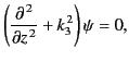
The mode frequencies are determined by the eigenvalues of
Equations (1329) and (1337). If we denote the functional dependence of
![]() or
or ![]() on the plane cross-section coordinates by
on the plane cross-section coordinates by ![]() then we can write Equation (1337) as
then we can write Equation (1337) as
| (1337) |
 |
(1338) |
 |
(1339) |
For TM modes, ![]() , and the
, and the ![]() dependence of
dependence of ![]() is given
by
is given
by
![]() . Equation (1338) must be solved subject to the
condition that
. Equation (1338) must be solved subject to the
condition that ![]() vanish on the boundaries of the plane cross-section,
thus completing the determination of
vanish on the boundaries of the plane cross-section,
thus completing the determination of ![]() and
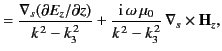
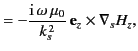
and ![]() . The transverse fields
are then given by special cases of Equations (1335)-(1336):
. The transverse fields
are then given by special cases of Equations (1335)-(1336):
For TE modes, in which ![]() , the condition that
, the condition that ![]() vanish at the
ends of the cylinder demands a
vanish at the
ends of the cylinder demands a
![]() dependence on
dependence on ![]() , and a
, and a ![]() which is
such that the normal derivative of
which is
such that the normal derivative of ![]() is zero at the walls.
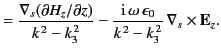
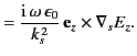
Equations (1335)-(1336), for the transverse fields, then become
is zero at the walls.
Equations (1335)-(1336), for the transverse fields, then become