


Next: Measurement of Ionospheric Electron
Up: Wave Propagation in Inhomogeneous
Previous: Extension to Oblique Incidence
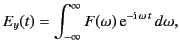
Consider a radio wave generator that launches radio pulses
vertically
upwards into the ionosphere. For the sake of argument, we shall assume that these
pulses are linearly polarized such that the electric field vector
lies parallel to the  -axis.
The pulse structure can be represented as
-axis.
The pulse structure can be represented as
 |
(1117) |
where  is the electric field produced by
the generator (i.e., the field at
is the electric field produced by
the generator (i.e., the field at  ).
Suppose that the pulse is a signal of roughly constant (angular)
frequency
).
Suppose that the pulse is a signal of roughly constant (angular)
frequency  that
lasts a time
that
lasts a time  , where
is long compared to
, where
is long compared to
 . It
follows that
. It
follows that  possesses narrow maxima around
 . In other words,
only those frequencies that lie very close to the central
frequency,
, play a significant role in the propagation of the pulse.
. In other words,
only those frequencies that lie very close to the central
frequency,
, play a significant role in the propagation of the pulse.
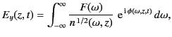
Each component frequency of the pulse yields a wave that travels independently
up into
the ionosphere, in a manner specified by the
appropriate WKB solution [see Equations (1104)-(1105)]. Thus, if Equation (1119)
specifies the signal at ground level (
) then the signal at height  is given by
 |
(1118) |
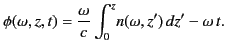
where
 |
(1119) |
Here, we have made use of the definition
 .
.
Equation (1120) can be regarded as a contour integral in  -space.
The quantity
-space.
The quantity
 is a relatively slowly varying function of
, whereas the phase
is a relatively slowly varying function of
, whereas the phase  is a large and rapidly varying
function. As described in Section 7.12, the rapid
oscillations of
is a large and rapidly varying
function. As described in Section 7.12, the rapid
oscillations of
 over most of the path of
integration ensure that the integrand averages almost to zero. However,
this cancellation argument does not apply to those points on the
integration path where the phase
is stationary: that is, where
over most of the path of
integration ensure that the integrand averages almost to zero. However,
this cancellation argument does not apply to those points on the
integration path where the phase
is stationary: that is, where
 .
It follows that the left-hand side of Equation (1120) averages to a very small
value, expect
for those special values of
and
.
It follows that the left-hand side of Equation (1120) averages to a very small
value, expect
for those special values of
and  at which one of the points of stationary
phase in
-space coincides with one of the peaks of
. The
locus of these special values of
and
can be regarded as the
equation of motion of the pulse as it propagates through the
ionosphere. Thus, the equation of motion is
specified by
at which one of the points of stationary
phase in
-space coincides with one of the peaks of
. The
locus of these special values of
and
can be regarded as the
equation of motion of the pulse as it propagates through the
ionosphere. Thus, the equation of motion is
specified by
 |
(1120) |
which yields
![$\displaystyle t = \frac{1}{c} \int_0^z \left[\frac{\partial(\omega \,n)}{\partial\omega} \right]_{\omega=\omega_0}\, dz'.$](img2338.png) |
(1121) |
Suppose that the
-velocity of a pulse of central frequency
at height
is given by
 . The differential
equation of motion of the pulse is then
. The differential
equation of motion of the pulse is then
 . This can be integrated,
using the boundary condition
at
. This can be integrated,
using the boundary condition
at  , to give the full equation
of motion:
, to give the full equation
of motion:
 |
(1122) |
A comparison between Equations (1123) and (1124) yields
![$\displaystyle u_z(\omega_0,z) = c\left/ \left\{\frac{\partial[\omega \,n(\omega,z)]}{\partial\omega} \right\}_{\omega=\omega_0}\right..$](img2342.png) |
(1123) |
The velocity  corresponds to the
group velocity of the pulse. (See Section 7.13.)
corresponds to the
group velocity of the pulse. (See Section 7.13.)
The dispersion relation (1056) yields
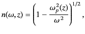 |
(1124) |
in the limit that electron collisions are negligible. The phase velocity
of radio waves of frequency
propagating vertically through the ionosphere is given
by
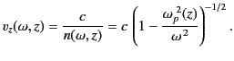 |
(1125) |
According to Equations (1125) and (1126), the corresponding group velocity
is
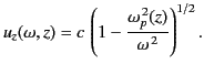 |
(1126) |
It follows that
 |
(1127) |
Note that as the reflection point  [defined as the root of
 ] is approached from below,
the phase velocity tends to infinity, whereas the group velocity tends
to zero.
] is approached from below,
the phase velocity tends to infinity, whereas the group velocity tends
to zero.
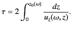
Let  be the time taken for the pulse to travel from the ground to the
reflection level, and then back to the ground again. The product
be the time taken for the pulse to travel from the ground to the
reflection level, and then back to the ground again. The product  is termed the equivalent height of reflection, and is denoted
 , because it is a function of the pulse frequency,
.
The equivalent height is the height at which an equivalent pulse traveling at the velocity
, because it is a function of the pulse frequency,
.
The equivalent height is the height at which an equivalent pulse traveling at the velocity  would have to
be reflected in order to have the same travel time as the actual pulse. Because we know that a
pulse of dominant frequency
propagates at height
with the
-velocity
would have to
be reflected in order to have the same travel time as the actual pulse. Because we know that a
pulse of dominant frequency
propagates at height
with the
-velocity
 (this is
true for both upgoing and downgoing pulses), and also that the pulse
is reflected at the height
(this is
true for both upgoing and downgoing pulses), and also that the pulse
is reflected at the height
 , where
, it
follows that
, where
, it
follows that
 |
(1128) |
Hence,
 |
(1129) |
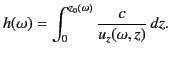
The equivalent height of reflection,
, is always greater than the
actual height of reflection,
, because the group velocity
is
always less than the velocity of light. The previous equation can be combined with
Equation (1128) to give
 |
(1130) |
Note that, despite the fact that the integrand diverges as the reflection point is approached,
the integral itself remains finite.
Next: Measurement of Ionospheric Electron
Up: Wave Propagation in Inhomogeneous
Previous: Extension to Oblique Incidence
Richard Fitzpatrick
2014-06-27