


Next: Brillouin Precursor
Up: Wave Propagation in Uniform
Previous: Method of Stationary Phase
Group Velocity
The point of stationary phase, defined by
 , satisfies the condition
 |
(918) |
where
 |
(919) |
is conventionally termed the group velocity. Thus, the signal
seen at position  and time
  is dominated by the frequency range
whose group velocity
is dominated by the frequency range
whose group velocity  is equal to
  . In this respect, the signal
incident at the surface of the medium (
. In this respect, the signal
incident at the surface of the medium ( ) at time
  can be said to propagate
through the medium at the group velocity
can be said to propagate
through the medium at the group velocity
 .
.
The simple one-resonance dielectric dispersion relation (871) yields
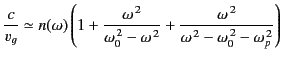 |
(920) |
in the limit
 ,
where
,
where
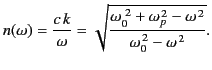 |
(921) |
The variation of  , and the refractive index
  , with frequency
is sketched in Figure 12. With
, with frequency
is sketched in Figure 12. With  , the group velocity
is less than
, the group velocity
is less than  for all
  , except for
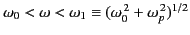 , where it is purely imaginary. Note that the
refractive index is also complex in this frequency range. The phase velocity
, where it is purely imaginary. Note that the
refractive index is also complex in this frequency range. The phase velocity
 is subluminal for
 , imaginary for
 , and superluminal for
 .
.
Figure:
The typical variation of the functions
 and
and
 . Here,
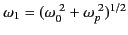 .
.
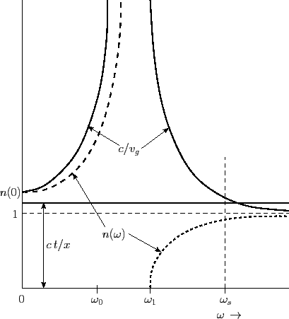 |
The frequency range that contributes to the amplitude at time
is determined graphically by finding the intersection of a horizontal
line with ordinate  with the solid curve in Figure 12. There is
no crossing of the two curves for
with the solid curve in Figure 12. There is
no crossing of the two curves for
 . Thus, no signal
can arrive before this time. For times immediately after
. Thus, no signal
can arrive before this time. For times immediately after  , the
point of stationary phase is seen to be at
, the
point of stationary phase is seen to be at
 .
In this large-
limit, the point of stationary phase satisfies
.
In this large-
limit, the point of stationary phase satisfies
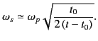 |
(922) |
Note that
 is also a point of stationary phase. It is
easily demonstrated that
is also a point of stationary phase. It is
easily demonstrated that
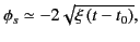 |
(923) |
and
 |
(924) |
with
 |
(925) |
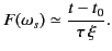
Here,  is given by Equation (894).
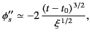
The stationary phase approximation (918) yields
is given by Equation (894).
The stationary phase approximation (918) yields
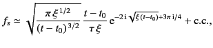 |
(926) |
where c.c. denotes the complex conjugate of the preceding term (this
contribution comes from the second point of stationary phase located at
). The previous expression reduces to
![$\displaystyle f_s \simeq \frac{ 2\sqrt{\pi}}{\tau} \,\frac{(t-t_0)^{1/4}}{\xi^{\,3/4}} \cos\!\left[2\sqrt{\xi\,(t-t_0)} - 3\pi/4\right].$](img1941.png) |
(927) |
It is readily shown that the previous formula is the same as
expression (903) for the Sommerfeld precursor in the large argument
limit
 .
Thus, the method of stationary phase yields an expression for the Sommerfeld
precursor that is accurate at all times except those immediately
following the first arrival of the signal.
.
Thus, the method of stationary phase yields an expression for the Sommerfeld
precursor that is accurate at all times except those immediately
following the first arrival of the signal.
Next: Brillouin Precursor
Up: Wave Propagation in Uniform
Previous: Method of Stationary Phase
Richard Fitzpatrick
2014-06-27