Retarded Potentials

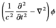
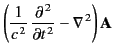
We are now in a position to solve Maxwell's equations. Recall, from Section 1.3, that Maxwell equations reduce to

$$\left(\frac{1}{c^{\,2}}\,\frac{\partial^{\,2}}{\partial t^{\,2}}-\nabla^{\,2}\right) \phi =\frac{\rho}{\epsilon_0},$$ (71)

$$\left(\frac{1}{c^{\,2}}\,\frac{\partial^{\,2}}{\partial t^{\,2}}-\nabla^{\,2} \right) {\bf A} = \mu_0 \,{\bf j}.$$ (72)

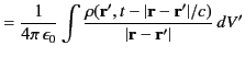
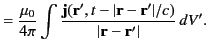
We can solve these inhomogeneous three-dimensional waves equations using the appropriate Green's function, (49). In fact, making use of Equation (46), we find that

$$\phi({\bf r},t) = \frac{1}{4\pi\,\epsilon_0} \int \frac{\rho({\bf r'}, t- \vert{\bf r} -{\bf r '}\vert/c)}{\vert{\bf r} - {\bf r}'\vert} \,dV'$$ (73)

$${\bf A}({\bf r}, t) = \frac{\mu_0}{4\pi } \int \frac{{\bf j}({\bf r'},t- \vert{\bf r} -{\bf r '}\vert/c )}{\vert{\bf r} - {\bf r}'\vert} \,dV'.$$ (74)

Alternatively, we can write

$$\phi({\bf r},t) = \frac{1}{4\pi \,\epsilon_0} \int \frac{\left[\rho({\bf r}')\right]}{\vert{\bf r} - {\bf r}'\vert}\,dV',$$ (75)

$${\bf A}({\bf r}, t) = \frac{\mu_0}{4\pi} \int \frac{\left[{\bf j}({\bf r}')\right]}{\vert{\bf r} - {\bf r}'\vert}\,dV'.$$ (76)

The above potentials are termed retarded potentials (because the integrands are evaluated at the retarded time). Finally, according to the discussion in the previous section, we can be sure that Equations (75) and (76) are the unique solutions to Equations (71) and (72), respectively, subject to sensible boundary conditions at infinity.