


Next: Cavities with Rectangular Boundaries
Up: Resonant Cavities and Waveguides
Previous: Introduction
The general boundary conditions on the field vectors
at an interface between medium 1 and medium 2 (say) are
where  is used for the interfacial surface change density (to avoid confusion
with the conductivity), and
is used for the interfacial surface change density (to avoid confusion
with the conductivity), and  is the surface current density.
Here,
is the surface current density.
Here,  is a unit vector normal to the interface, directed
from medium 2 to medium 1. We saw in Section 7.4 that, at normal
incidence, the amplitude of an electromagnetic wave falls off very rapidly with distance inside the
surface of a good conductor. In the
limit of perfect conductivity (i.e.,
is a unit vector normal to the interface, directed
from medium 2 to medium 1. We saw in Section 7.4 that, at normal
incidence, the amplitude of an electromagnetic wave falls off very rapidly with distance inside the
surface of a good conductor. In the
limit of perfect conductivity (i.e.,
 ), the wave does not penetrate into the conductor
at all, in which case the internal tangential electric and magnetic fields vanish. This implies, from
Equations (1297) and (1299), that the tangential component
of
), the wave does not penetrate into the conductor
at all, in which case the internal tangential electric and magnetic fields vanish. This implies, from
Equations (1297) and (1299), that the tangential component
of  vanishes just outside the surface of a
good conductor, whereas the tangential component of
vanishes just outside the surface of a
good conductor, whereas the tangential component of  may
remain finite.
Let us examine the behavior of the normal field components.
may
remain finite.
Let us examine the behavior of the normal field components.
Let medium 1 be a conductor, of conductivity  and dielectric constant
 , for which
 , and let medium 2 be a perfect insulator of dielectric constant
 . The change density
that forms at the interface between the two media
is related to the currents flowing inside the conductor. In fact, the
conservation of charge requires that
. The change density
that forms at the interface between the two media
is related to the currents flowing inside the conductor. In fact, the
conservation of charge requires that
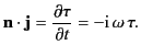 |
(1298) |
However,
 ,
so it follows from Equation (1296) that
,
so it follows from Equation (1296) that
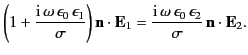 |
(1299) |
Thus, it is clear that the normal component of
within the conductor
also becomes vanishingly small as the conductivity approaches
infinity.
If
vanishes inside a perfect conductor then the curl of
also vanishes, and the time rate of change of  is correspondingly
zero. This implies that there are no oscillatory fields whatever inside
such a conductor, and that the fields just outside
satisfy
is correspondingly
zero. This implies that there are no oscillatory fields whatever inside
such a conductor, and that the fields just outside
satisfy
Here,
is a unit normal at the surface of the conductor
pointing into the conductor.
Thus, the electric field is normal, and the magnetic field tangential,
at the surface of a perfect conductor. For good conductors, these boundary
conditions yield excellent representations of the geometrical
configurations of the external fields, but they lead to the neglect of
some important features of real fields, such as losses in cavities
and signal attenuation in waveguides.
In order to estimate such losses, it is helpful to examine how the tangential
and normal fields compare when
is large but finite. Equations (773) and (808) imply that
 |
(1304) |
at the surface of a good conductor (provided that the wave propagates into
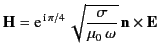
the conductor). Let us assume, without obtaining a complete
solution, that a wave with
very nearly tangential
and
very nearly normal propagates parallel to the surface of a good conductor. According to the Faraday-Maxwell equation,
 |
(1305) |
just outside the surface,
where  is the component of the wavevector parallel to the surface.
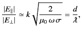
However, Equation (1306) implies that a tangential component of
is accompanied by a small tangential component of
. By comparing
the previous two expressions, we obtain
is the component of the wavevector parallel to the surface.
However, Equation (1306) implies that a tangential component of
is accompanied by a small tangential component of
. By comparing
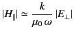
the previous two expressions, we obtain
 |
(1306) |
where  is the skin depth [see Equation (810)] and
 . It is clear that the ratio of the tangential to the normal component of
is of order the skin depth divided by the wavelength.
It is readily demonstrated that the ratio of the normal to the tangential component of
is of the same order of magnitude. Thus, we deduce that,
in the limit of high conductivity, which implies vanishing skin depth,
no fields penetrate into the conductor, and the boundary conditions are those
given by Equations (1302)-(1305). Let us investigate the solution of the homogeneous
wave equation subject to such constraints.
. It is clear that the ratio of the tangential to the normal component of
is of order the skin depth divided by the wavelength.
It is readily demonstrated that the ratio of the normal to the tangential component of
is of the same order of magnitude. Thus, we deduce that,
in the limit of high conductivity, which implies vanishing skin depth,
no fields penetrate into the conductor, and the boundary conditions are those
given by Equations (1302)-(1305). Let us investigate the solution of the homogeneous
wave equation subject to such constraints.
Next: Cavities with Rectangular Boundaries
Up: Resonant Cavities and Waveguides
Previous: Introduction
Richard Fitzpatrick
2014-06-27