Next: Antenna Directivity and Effective
Up: Radiation and Scattering
Previous: Introduction
It possible to solve exactly for the radiation pattern
emitted by a
linear antenna fed with a sinusoidal current pattern.
Assuming that all fields and currents vary in time like
 , and adopting the Lorenz gauge,
it is easily demonstrated that the vector potential obeys the inhomogeneous
Helmholtz equation,
, and adopting the Lorenz gauge,
it is easily demonstrated that the vector potential obeys the inhomogeneous
Helmholtz equation,
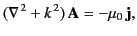 |
(1213) |
where
 .
The Green's function for
this equation, subject to the Sommerfeld radiation
condition (which ensures that sources radiate waves instead of absorbing
them),
is
.
The Green's function for
this equation, subject to the Sommerfeld radiation
condition (which ensures that sources radiate waves instead of absorbing
them),
is
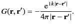 |
(1214) |
(See Chapter 1.)
Thus, we can invert Equation (1215) to obtain
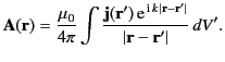 |
(1215) |
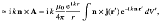
The electric field in the source-free region,
 |
(1216) |
follows from the Ampère-Maxwell
equation, as well as the definition
 ,
,
Now,
![$\displaystyle \vert{\bf r} - {\bf r}'\vert = r\left[1- \frac{2\,{\bf n}\cdot{\bf r}'}{r}+ \frac{{r'}^{\,2}}{r^{\,2}}\right]^{1/2},$](img2601.png) |
(1217) |
where
 .
Assuming that
.
Assuming that  , this expression can be expanded binomially to
give
, this expression can be expanded binomially to
give
![$\displaystyle \vert{\bf r} -{\bf r}'\vert = r\left[ 1-\frac{{\bf n}\cdot{\bf r}...
...}} -\frac{1}{8}\left(\frac{2\,{\bf n}\cdot{\bf r}'}{r}\right)^2 +\cdots\right],$](img2604.png) |
(1218) |
where we have retained all terms up to order
 . The above expansion, which appears in the complex exponential of Equation (1217),
determines the phase of the radiation emitted by each element of the
antenna. The quadratic terms in the expansion can be neglected provided
they can be shown to contribute a phase change that is significantly
less than
. The above expansion, which appears in the complex exponential of Equation (1217),
determines the phase of the radiation emitted by each element of the
antenna. The quadratic terms in the expansion can be neglected provided
they can be shown to contribute a phase change that is significantly
less than  . Thus, because the maximum possible value of
  is
is  ,
for a linear antenna that extends along the
,
for a linear antenna that extends along the  -axis from
  to
to
 , the phase shift associated with the quadratic
terms is insignificant as long as
, the phase shift associated with the quadratic
terms is insignificant as long as
 |
(1219) |
where
 is the wavelength of the radiation. This constraint
is known as the Fraunhofer limit.
is the wavelength of the radiation. This constraint
is known as the Fraunhofer limit.
In the Fraunhofer limit, we can approximate the phase variation
of the complex exponential in Equation (1217) as a linear function of
:
 |
(1220) |
The denominator
 in the integrand of
Equation (1217) can be approximated as
in the integrand of
Equation (1217) can be approximated as  provided
that the distance from the antenna is much greater than its length:
that is,
provided
that the distance from the antenna is much greater than its length:
that is,
 |
(1221) |
Thus, Equation (1217)
reduces to
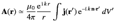 |
(1222) |
when the constraints (1221) and (1223) are satisfied. If the additional
constraint
 |
(1223) |
is also satisfied then the electromagnetic fields associated with Equation (1224)
take the form
These are clearly radiation fields, because they are mutually orthogonal,
transverse to the radius vector,  , and satisfy
 . (See Section 1.8.)
The three constraints (1221), (1223), and (1225), can be summed up
in the single inequality
. (See Section 1.8.)
The three constraints (1221), (1223), and (1225), can be summed up
in the single inequality
 |
(1226) |
The current density associated with a linear, sinusoidal,
centre-fed antenna, aligned along the
-axis, is
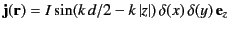 |
(1227) |
for  , with
 for
for
 . In this case, Equation (1224)
yields
. In this case, Equation (1224)
yields
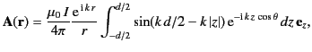 |
(1228) |
where
 . The result of this
straightforward integration is
. The result of this
straightforward integration is
![$\displaystyle {\bf A}({\bf r}) =\frac{\mu_0\, I}{4\pi} \frac{2\,{\rm e}^{\,{\rm...
...t[\frac{\cos(k\,d \,\cos\theta/2) -\cos(k\,d/2)}{\sin^2\theta}\right]{\bf e}_z.$](img2627.png) |
(1229) |
According to Equations (1226) and (1227), the electric component of the emitted radiation lies in the plane containing
the antenna and the radius vector connecting the antenna to the observation point.
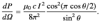
The time-averaged power radiated by the antenna per unit solid angle
is
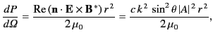 |
(1230) |
or
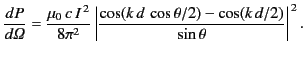 |
(1231) |
The angular distribution of power depends on the value of
 . In the long wavelength limit,
  , the distribution
reduces to
, the distribution
reduces to
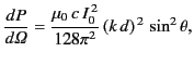 |
(1232) |
where
 is the peak current in the antenna. It is easily
shown, from Equation (1229), that the associated current distribution in the antenna is linear: that is,
is the peak current in the antenna. It is easily
shown, from Equation (1229), that the associated current distribution in the antenna is linear: that is,
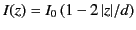 |
(1233) |
for
. This type of antenna corresponds to a short (compared to
the wavelength) oscillating
electric dipole, and is generally known
as a Hertzian dipole. The total power radiated is
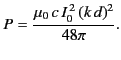 |
(1234) |
In order to maintain the radiation, power must be supplied continuously
to the dipole from some generator. By analogy with the
heating power produced in a resistor,
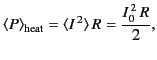 |
(1235) |
we can define the factor which multiplies
 in Equation (1236)
as the radiation resistance of the dipole antenna. Hence,
in Equation (1236)
as the radiation resistance of the dipole antenna. Hence,
 |
(1236) |
Because we have assumed that
 , this radiation resistance
is necessarily small. Typically, in a Herztian dipole, the
radiated power is swamped by ohmic losses that appear as heat.
Thus, a ``short'' antenna is a very inefficient radiator. Practical
antennas have dimensions that are comparable with the wavelength of the
emitted radiation.
, this radiation resistance
is necessarily small. Typically, in a Herztian dipole, the
radiated power is swamped by ohmic losses that appear as heat.
Thus, a ``short'' antenna is a very inefficient radiator. Practical
antennas have dimensions that are comparable with the wavelength of the
emitted radiation.
Probably the two most common practical antennas are the half-wave antenna
( ) and the full-wave antenna (
 ). In the former case,
Equation (1233) reduces to
). In the former case,
Equation (1233) reduces to
 |
(1237) |
In the latter case, Equation (1233) yields
 |
(1238) |
The half-wave antenna radiation pattern
is very similar to the characteristic
 pattern of
a Hertzian dipole. However, the full-wave antenna radiation pattern
is considerably sharper (i.e., it is more concentrated in the
transverse directions
pattern of
a Hertzian dipole. However, the full-wave antenna radiation pattern
is considerably sharper (i.e., it is more concentrated in the
transverse directions
 ).
).
The total power radiated by a half-wave antenna is
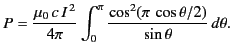 |
(1239) |
The integral can be evaluated numerically to give  . Thus,
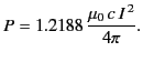 |
(1240) |
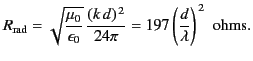
Note, from Equation (1229), that  is
equivalent to the peak current flowing in the antenna. Thus, the radiation
resistance of a half-wave antenna is given by
is
equivalent to the peak current flowing in the antenna. Thus, the radiation
resistance of a half-wave antenna is given by
 , or
, or
 |
(1241) |
This resistance is substantially larger than that of a
Hertzian dipole [see Equation (1238)]. In other words, a half-wave antenna
is a far more efficient emitter of electromagnetic radiation than a
Hertzian dipole.
According to standard transmission line
theory, if a transmission line is terminated by a resistor whose resistance
matches the characteristic impedance of the line then all of the power transmitted down the line is dissipated in the resistor. On the other hand, if the
resistance does not match the impedance of the line then some
of the power is reflected and returned to the generator. We can think of a
half-wave antenna, centre-fed by a transmission line, as a 73 ohm resistor
terminating the line. The only difference is that the power absorbed from
the line is radiated rather than dissipated as heat.
Thus, in order to avoid problems with reflected power,
the impedance of a transmission line feeding a half-wave
antenna must be 73 ohms. Not surprisingly, 73 ohm impedance
is one of the standard ratings for the co-axial cables used in amateur
radio.
Next: Antenna Directivity and Effective
Up: Radiation and Scattering
Previous: Introduction
Richard Fitzpatrick
2014-06-27