Momentum conservation

It follows from Eqs. (1036) and (1050) that the momentum density of electromagnetic fields can be written

$${\bf g} = \epsilon_0 {\bf E}\times{\bf B}.$$ (1058)

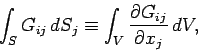
Now, a momentum conservation equation for electromagnetic fields should take the integral form

$$-\frac{\partial}{\partial t}\int_V g_i dV = \int_S G_{ij} ... ...int_V \left[\rho {\bf E} + {\bf j}\times{\bf B}\right]_i dV.$$ (1059)

Here, $i$ and $j$ run from 1 to 3 (1 corresponds to the $x$-direction, 2 to the $y$-direction, and 3 to the $z$-direction). Moreover, the Einstein summation convention is employed for repeated indices (e.g., $a_j a_j\equiv {\bf a}\cdot{\bf a}$). Furthermore, the tensor $G_{ij}$ represents the flux of the $i$th component of electromagnetic momentum in the $j$-direction. This tensor (a tensor is a direct generalization of a vector with two indices instead of one) is called the momentum flux density. Hence, the above equation states that the rate of loss of electromagnetic momentum in some volume $V$ is equal to the flux of electromagnetic momentum across the bounding surface $S$ plus the rate at which momentum is transferred to matter inside $V$. The latter rate is, of course, just the net electromagnetic force acting on matter inside $V$: i.e., the volume integral of the electromagnetic force density, $\rho {\bf E} + {\bf j}\times{\bf B}$. Now, a direct generalization of the divergence theorem states that

$$\int_S G_{ij} dS_j \equiv \int_V \frac {\partial G_{ij}}{\partial x_j} dV,$$ (1060)

where $x_1 \equiv x$, $x_2\equiv y$, etc. Hence, in differential form, our momentum conservation equation for electromagnetic fields is written

$$-\frac{\partial}{\partial t}\left[\epsilon_0 {\bf E}\times{... ...ij}}{\partial x_j} + [\rho {\bf E} + {\bf j}\times{\bf B}]_i.$$ (1061)

Let us now attempt to derive an equation of this form from Maxwell's equations.

Maxwell's equations are written:

$$\nabla\cdot{\bf E} = \frac{\rho}{\epsilon_0},$$ (1062)

$$\nabla\cdot{\bf B} = 0,$$ (1063)

$$\nabla\times{\bf E} = - \frac{\partial {\bf B}}{\partial t} ,$$ (1064)

$$\nabla\times{\bf B} = \mu_0 {\bf j} + \epsilon_0\mu_0 \frac{\partial {\bf E}}{\partial t}.$$ (1065)

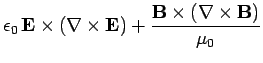
We can cross Eq. (1065) divided by $\mu_0$ with ${\bf B}$, and rearrange, to give

$$-\epsilon_0 \frac{\partial {\bf E}}{\partial t}\times {\bf ... ...}\times(\nabla\times {\bf B})}{\mu_0} + {\bf j}\times {\bf B}.$$ (1066)

Next, let us cross ${\bf E}$ with Eq. (1064) times $\epsilon_0$, rearrange, and add the result to the above equation. We obtain

$$-\epsilon_0 \frac{\partial {\bf E}}{\partial t}\times {\bf ... ...}\times(\nabla\times {\bf B})}{\mu_0} + {\bf j}\times {\bf B}.$$ (1067)

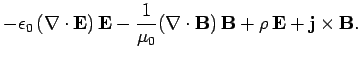
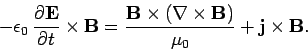
Next, making use of Eqs. (1062) and (1063), we get

$$-\frac{\partial}{\partial t} \left[\epsilon_0 {\bf E}\times{\bf B}\right] = \epsilon_0 {\bf E}\times (\nabla\times{\bf E})+\frac{{\bf B}\times(\nabla\times {\bf B})}{\mu_0}$$

$$- \epsilon_0 (\nabla\cdot {\bf E}) {\bf E} - \frac{1}{\mu_0}(\nabla\cdot {\bf B}) {\bf B}+ \rho {\bf E}+{\bf j}\times {\bf B}.$$ (1068)

Now, from vector field theory,

$$\nabla (E^2/2) \equiv {\bf E}\times(\nabla\times {\bf E}) + ({\bf E}\cdot{\nabla}){\bf E},$$ (1069)

with a similar equation for ${\bf B}$. Hence, Eq. (1068) takes the form

$$-\frac{\partial}{\partial t} \left[\epsilon_0 {\bf E}\times{\bf B}\right] = \epsilon_0\left[\nabla(E^2/2) - (\nabla\cdot {\bf E}) {\bf E} - ({\bf E}\cdot\nabla){\bf E}\right]$$

$$+\frac{1}{\mu_0}\left[\nabla(B^2/2) - (\nabla\cdot {\bf B}) {\bf B} - ({\bf B}\cdot\nabla){\bf B}\right]$$

$$+ \rho {\bf E}+{\bf j}\times {\bf B}.$$ (1070)

Finally, when written in terms of components, the above equation becomes

$$-\frac{\partial}{\partial t} \left[\epsilon_0 {\bf E}\times{\bf B}\right]_i = \frac{\partial}{\partial x_j}\!\left[\epsilon_0 E^2 \delta_{ij}/2 - \epsilon_0 E_i E_j+ B^2 \delta_{ij}/2 \mu_0 - B_i B_j/\mu_0\right]$$

$$+ \left[\rho {\bf E}+{\bf j}\times {\bf B}\right]_i,$$ (1071)

since $[(\nabla\cdot{\bf E}) {\bf E}]_i = (\partial E_j/\partial x_j) E_i$, and $[({\bf E}\cdot\nabla){\bf E}]_i = E_j (\partial E_i/\partial x_j)$. Here, $\delta_{ij}$ is a Kronecker delta symbol (i.e., $\delta_{ij}=1$ if $i=j$, and $\delta_{ij}=0$ otherwise). Comparing the above equation with Eq. (1061), we conclude that the momentum flux density tensor of electromagnetic fields takes the form

$$G_{ij} = \epsilon_0 (E^2 \delta_{ij}/2-E_i E_j) + (B^2 \delta_{ij}/2-B_i B_j)/ \mu_0.$$ (1072)

The momentum conservation equation (1061) is sometimes written

$$[\rho {\bf E} + {\bf j}\times{\bf B}]_i = \frac {\partial T_... ...l}{\partial t}\left[\epsilon_0 {\bf E}\times{\bf B}\right]_i,$$ (1073)

where

$$T_{ij} = - G_{ij} = \epsilon_0 (E_i E_j-E^2 \delta_{ij}/2) + (B_i B_j-B^2 \delta_{ij}/2)/ \mu_0$$ (1074)

is called the Maxwell stress tensor.