


Next: Mutual inductance
Up: Magnetic induction
Previous: Inductance
Consider a long solenoid of length  , and radius
  ,
which has
,
which has  turns per unit length,
and carries a current
turns per unit length,
and carries a current  . The longitudinal (i.e., directed along the
axis of the solenoid) magnetic field within the solenoid is approximately uniform,
and is given by
. The longitudinal (i.e., directed along the
axis of the solenoid) magnetic field within the solenoid is approximately uniform,
and is given by
 |
(907) |
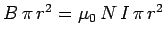
This result is easily obtained by integrating Ampère's law over a rectangular
loop whose long sides run parallel to the axis of the solenoid, one inside the
solenoid, and the other outside, and whose short sides run perpendicular to the
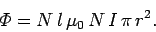
axis. The magnetic flux though each turn of the loop is
 . The total flux through
the solenoid wire, which has
. The total flux through
the solenoid wire, which has  turns, is
 |
(908) |
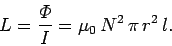
Thus, the self-inductance of the solenoid is
 |
(909) |
Note that the self-inductance only depends on geometric quantities such as the number
of turns per unit length of the solenoid, and the cross-sectional area of the turns.
Suppose that the current flowing through the solenoid changes. We have to
assume that the change is sufficiently slow that we can neglect the displacement
current, and retardation effects, in our calculations. This implies that the typical
time-scale of the change must be much longer than the time for a light-ray to traverse the
circuit. If this is the case, then the above formulae remain valid.
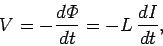
A change in the current implies a change in the magnetic flux linking the solenoid
wire, since
 . According to Faraday's
law, this change
generates an e.m.f. in the wire. By Lenz's law, the e.m.f. is such
as to oppose the change in the current--i.e., it is a back e.m.f. We can write
. According to Faraday's
law, this change
generates an e.m.f. in the wire. By Lenz's law, the e.m.f. is such
as to oppose the change in the current--i.e., it is a back e.m.f. We can write
 |
(910) |
where  is the generated e.m.f.
Figure 51:
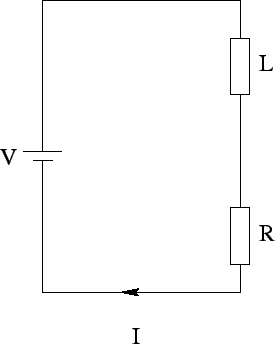 |
Suppose that our solenoid has an electrical resistance  . Let us
connect the ends of the solenoid across the terminals of a battery of
e.m.f. . What is going to happen? The equivalent circuit is shown in Fig. 51.
The inductance and resistance of the solenoid are represented by a perfect
inductor,
. Let us
connect the ends of the solenoid across the terminals of a battery of
e.m.f. . What is going to happen? The equivalent circuit is shown in Fig. 51.
The inductance and resistance of the solenoid are represented by a perfect
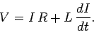
inductor,  , and a perfect resistor, , connected in series. The voltage drop
across the inductor and resistor is equal to the e.m.f. of the battery,
. The voltage drop across the resistor is simply
, and a perfect resistor, , connected in series. The voltage drop
across the inductor and resistor is equal to the e.m.f. of the battery,
. The voltage drop across the resistor is simply  , whereas the
voltage drop across the inductor (i.e., the back e.m.f.) is
, whereas the
voltage drop across the inductor (i.e., the back e.m.f.) is
 . Here, is the current flowing through the solenoid.
It follows that
. Here, is the current flowing through the solenoid.
It follows that
 |
(911) |
This is a differential equation for the current . We can rearrange it to
give
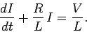 |
(912) |
The general solution is
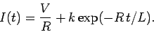 |
(913) |
The constant  is fixed by the boundary conditions. Suppose that the
battery is connected at time
is fixed by the boundary conditions. Suppose that the
battery is connected at time  , when
  . It follows that
  , so
that
, so
that
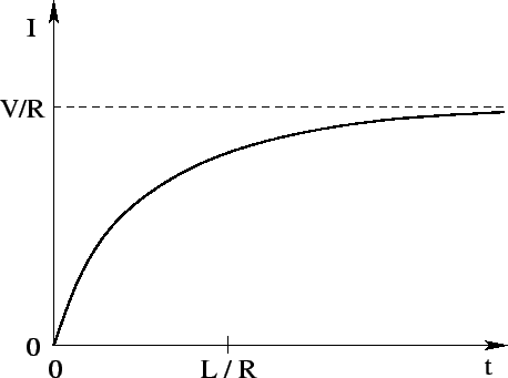
![\begin{displaymath}
I(t) = \frac{V}{R} \left[1-\exp(-R t/L) \right].
\end{displaymath}](img1901.png) |
(914) |
This curve is sketched in Fig. 52. It can be seen that, after the battery is connected, the current
ramps up, and attains its steady-state value  (which comes from Ohm's
law), on the characteristic time-scale
(which comes from Ohm's
law), on the characteristic time-scale
 |
(915) |
This time-scale is sometimes called the time constant of the circuit, or,
somewhat unimaginatively, the L over R time of the circuit.
Figure 52:
 |
We can now appreciate the significance of self-inductance. The back e.m.f.
generated in an inductor, as the current tries to change, effectively prevents the
current from rising (or falling) much faster than the  time. This effect is
sometimes advantageous, but often it is a great nuisance.
All circuit elements possess some self-inductance, as well as some resistance, and thus have a finite time. This means that when we power up a circuit, the current
does not jump up instantaneously to its steady-state value. Instead, the
rise is spread out over the L/R time of the circuit. This is a good thing.
If the current were to rise instantaneously, then extremely large electric
fields would be generated by the sudden jump in the induced magnetic field, leading,
inevitably, to breakdown and electric arcing. So, if there were no such thing
as self-inductance, then every time you switched an electric circuit on or off
there would be a blue flash due to arcing between conductors. Self-inductance
can also be a bad thing. Suppose that we possess a fancy power supply, and we wish
to use it to send an electric signal down a wire (or transmission line).
Of course, the wire or transmission line will possess both resistance and inductance,
and will, therefore, have some characteristic time. Suppose that we
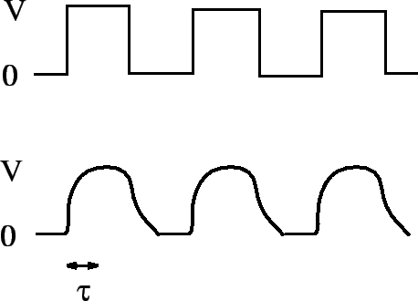
try to send a square-wave signal down the wire. Since the current in the wire
cannot rise or fall faster than the time, the leading and trailing edges of
the signal get smoothed out over an time. The typical difference between
the signal fed into the wire (upper trace), and that which comes out of the
other end (lower trace), is illustrated in Fig. 53. Clearly, there is little
point having a fancy power supply unless you also possess a low inductance
wire or transmission line, so that the signal from the power supply can be
transmitted to some load device without serious distortion.
time. This effect is
sometimes advantageous, but often it is a great nuisance.
All circuit elements possess some self-inductance, as well as some resistance, and thus have a finite time. This means that when we power up a circuit, the current
does not jump up instantaneously to its steady-state value. Instead, the
rise is spread out over the L/R time of the circuit. This is a good thing.
If the current were to rise instantaneously, then extremely large electric
fields would be generated by the sudden jump in the induced magnetic field, leading,
inevitably, to breakdown and electric arcing. So, if there were no such thing
as self-inductance, then every time you switched an electric circuit on or off
there would be a blue flash due to arcing between conductors. Self-inductance
can also be a bad thing. Suppose that we possess a fancy power supply, and we wish
to use it to send an electric signal down a wire (or transmission line).
Of course, the wire or transmission line will possess both resistance and inductance,
and will, therefore, have some characteristic time. Suppose that we
try to send a square-wave signal down the wire. Since the current in the wire
cannot rise or fall faster than the time, the leading and trailing edges of
the signal get smoothed out over an time. The typical difference between
the signal fed into the wire (upper trace), and that which comes out of the
other end (lower trace), is illustrated in Fig. 53. Clearly, there is little
point having a fancy power supply unless you also possess a low inductance
wire or transmission line, so that the signal from the power supply can be
transmitted to some load device without serious distortion.
Figure 53:
 |
Next: Mutual inductance
Up: Magnetic induction
Previous: Inductance
Richard Fitzpatrick
2006-02-02