Magnetic energy

Consider an electrical conductor. Suppose that a battery with an electromotive field ${\bf E}'$ is feeding energy into this conductor. The energy is either dissipated as heat, or is used to generate a magnetic field. Ohm's law inside the conductor gives

$${\bf j}_t = \sigma ({\bf E} + {\bf E}'),$$ (886)

where ${\bf j}_t$ is the true current density, $\sigma$ is the conductivity, and ${\bf E}$ is the inductive electric field. Taking the scalar product with ${\bf j}_t$, we obtain

$${\bf E}'\!\cdot\!{\bf j}_t = \frac{j_t^{ 2}}{\sigma} -{\bf E}\!\cdot\!{\bf j}_t.$$ (887)

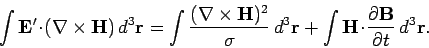
The left-hand side of this equation represents the rate at which the battery does work on the conductor. The first term on the right-hand side is the rate of ohmic heating inside the conductor. We tentatively identify the remaining term with the rate at which energy is fed into the magnetic field. If all fields are quasi-stationary (i.e., slowly varying) then the displacement current can be neglected, and the differential form of Ampère's law reduces to $\nabla\times{\bf H} = {\bf j}_t$. Substituting this expression into Eq. (887), and integrating over all space, we get

$$\int {\bf E}'\!\cdot\!(\nabla\times{\bf H}) d^3{\bf r} = \i... ... r} - \int {\bf E}\!\cdot\!(\nabla\times{\bf H}) d^3{\bf r}.$$ (888)

The last term can be integrated by parts using the vector identity

$$\nabla\!\cdot\!({\bf E}\times{\bf H}) \equiv {\bf H}\!\cdot\!(\nabla\times {\bf E}) - {\bf E}\!\cdot\!(\nabla\times{\bf H}).$$ (889)

Gauss' theorem plus the differential form of Faraday's law yield

$$\int{\bf E}\!\cdot\!(\nabla\times{\bf H}) d^3{\bf r} = -\i... ... t} d^3{\bf r} - \int({\bf E}\times{\bf H})\!\cdot\!d{\bf S}.$$ (890)

Since ${\bf E}\times{\bf H}$ falls off at least as fast as $1/r^5$ in electrostatic and quasi-stationary magnetic fields ($1/r^2$ comes from electric monopole fields, and $1/r^3$ from magnetic dipole fields), the surface integral in the above expression can be neglected. Of course, this is not the case for radiation fields, for which ${\bf E}$ and ${\bf H}$ fall off like $1/r$. Thus, the constraint of ``quasi-stationarity'' effectively means that the fields vary sufficiently slowly that any radiation fields can be neglected.

The total power expended by the battery can now be written

$$\int {\bf E}'\!\cdot\!(\nabla\times{\bf H}) d^3{\bf r} = \i... ...bf H}\!\cdot\!\frac{\partial{\bf B}}{\partial t} d^3{\bf r}.$$ (891)

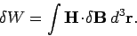
The first term on the right-hand side has already been identified as the energy loss rate due to ohmic heating. The last term is obviously the rate at which energy is fed into the magnetic field. The variation $\delta W$ in the magnetic field energy can therefore be written

$$\delta W = \int {\bf H}\!\cdot\!\delta {\bf B} d^3{\bf r}.$$ (892)

This result is analogous to the result (851) for the variation in the energy of an electrostatic field.

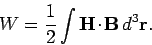
In order to make Eq. (892) integrable, we must assume a functional relationship between ${\bf H}$ and ${\bf B}$. For a medium which magnetizes linearly, the integration can be carried out in much the same manner as Eq. (854), to give

$$W = \frac{1}{2} \int {\bf H}\!\cdot\!{\bf B} d^3{\bf r}.$$ (893)

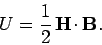
Thus, the magnetostatic energy density inside a linear magnetic material is given by

$$U=\frac{1}{2} {\bf H}\!\cdot{\bf B}.$$ (894)

Unfortunately, most interesting magnetic materials, such as ferromagnets, exhibit a nonlinear relationship between ${\bf H}$ and ${\bf B}$. For such materials, Eq. (892) can only be integrated between definite states, and the result, in general, depends on the past history of the sample. For ferromagnets, the integral of Eq. (892) has a finite, non-zero value when ${\bf B}$ is integrated around a complete magnetization cycle. This cyclic energy loss is given by

$$\Delta W = \int \oint {\bf H}\!\cdot d{\bf B} d^3{\bf r}.$$ (895)

In other words, the energy expended per unit volume when a magnetic material is carried through a magnetization cycle is equal to the area of its hysteresis loop, as plotted in a graph of $B$ against $H$. Thus, it is particularly important to ensure that the magnetic materials used to form transformer cores possess hysteresis loops with comparatively small areas, otherwise the transformers are likely to be extremely lossy.