Next: Energy density within a
Up: Dielectric and magnetic media
Previous: Boundary conditions for and
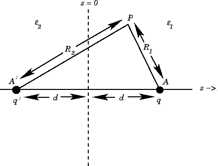
Consider a point charge  embedded in a semi-infinite dielectric
 a distance
  away from a plane interface which
separates the first medium from another semi-infinite dielectric
away from a plane interface which
separates the first medium from another semi-infinite dielectric
 . The interface is assumed to coincide with the plane
  .
We need to find solutions to the equations
.
We need to find solutions to the equations
 |
(818) |
for  ,
,
 |
(819) |
for  , and
, and
 |
(820) |
everywhere, subject to the boundary conditions at that
Figure 47:
 |
In order to solve this problem, we shall employ a slightly modified form of
the well-known method of images. Since
 everywhere,
the electric field can be written in terms of a scalar potential.
So,
everywhere,
the electric field can be written in terms of a scalar potential.
So,
 . Consider the region .
Let us assume that the scalar potential in this region is the same as
that obtained when the whole of space is filled with the dielectric
, and, in addition to the real charge at position
. Consider the region .
Let us assume that the scalar potential in this region is the same as
that obtained when the whole of space is filled with the dielectric
, and, in addition to the real charge at position  ,
there is a second charge
,
there is a second charge  at the image position
  (see Fig. 47).
If this is the case, then the potential at some point
(see Fig. 47).
If this is the case, then the potential at some point  in the region is given by
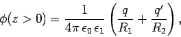 |
(824) |
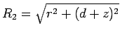
where
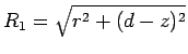 and
and
 , when
written in terms of cylindrical polar coordinates,
, when
written in terms of cylindrical polar coordinates,
 , aligned along the
  -axis.
Note that the potential (824) is clearly a solution of Eq. (818) in
the region . It gives
-axis.
Note that the potential (824) is clearly a solution of Eq. (818) in
the region . It gives
 , with the
appropriate singularity at the position of the point charge .
, with the
appropriate singularity at the position of the point charge .
Consider the region . Let us assume that the scalar potential in this
region is the same as that obtained when the whole of space is filled
with the dielectric , and a charge  is located at the point
. If this is the case, then the potential in this region is
given by
is located at the point
. If this is the case, then the potential in this region is
given by
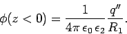 |
(825) |
The above potential is clearly a solution of Eq. (819) in the region
. It gives
 , with
no singularities.
, with
no singularities.
It now remains to choose and in such a manner that the boundary
conditions (821)-(823) are satisfied. The boundary conditions (822) and
(823) are obviously satisfied if the scalar potential is continuous
at the interface between the two dielectric media:
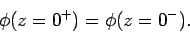 |
(826) |
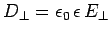
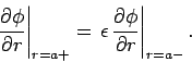
The boundary condition (821) implies a jump in the normal derivative
of the scalar potential across the interface:
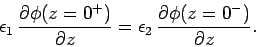 |
(827) |
The first matching condition yields
 |
(828) |
whereas the second gives
 |
(829) |
Here, use has been made of
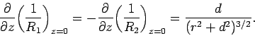 |
(830) |
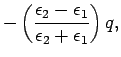
Equations (828) and (829) imply that
The bound charge density is given by
 , However, inside either dielectric,
 , so
, so
 , except at the point charge .
Thus, there is zero bound charge density in either dielectric
medium. However,
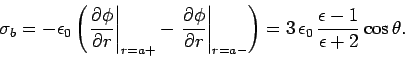
there is a bound charge sheet on the interface
between the two dielectric media.
In fact, the density of this sheet is given by
, except at the point charge .
Thus, there is zero bound charge density in either dielectric
medium. However,
there is a bound charge sheet on the interface
between the two dielectric media.
In fact, the density of this sheet is given by
 |
(833) |
Hence,
 |
(834) |
In the limit
 , the dielectric
behaves like a conducting medium (i.e.,
, the dielectric
behaves like a conducting medium (i.e.,
 in the region ), and the bound surface charge density
on the interface approaches that obtained in the case where the plane
coincides with a conducting surface (see Sect. 5.10).
in the region ), and the bound surface charge density
on the interface approaches that obtained in the case where the plane
coincides with a conducting surface (see Sect. 5.10).
As a second example, consider a dielectric sphere of radius  , and
uniform dielectric constant
, and
uniform dielectric constant  , placed in a uniform
-directed electric field of magnitude
, placed in a uniform
-directed electric field of magnitude  . Suppose that the
sphere is centered on the origin. Now, for an electrostatic problem, we
can always write
. In the present problem,
. Suppose that the
sphere is centered on the origin. Now, for an electrostatic problem, we
can always write
. In the present problem,
 both inside and outside the sphere, since there are no free charges, and the bound volume charge density is zero in a uniform
dielectric medium (or a vacuum). Hence, the scalar potential satisfies Laplace's equation,
both inside and outside the sphere, since there are no free charges, and the bound volume charge density is zero in a uniform
dielectric medium (or a vacuum). Hence, the scalar potential satisfies Laplace's equation,
 , throughout space. Adopting spherical polar coordinates,
 , aligned along the -axis, the boundary conditions are that
 at
at
 , and that
  is well-behaved at
 . At the surface of the sphere,
  , the continuity of
  implies that is continuous. Furthermore, the
continuity of
implies that is continuous. Furthermore, the
continuity of
 leads to the matching condition
 |
(835) |
Let us try separable solutions of the form
 . It is
easily demonstrated that such solutions satisfy Laplace's equation
provided that
. It is
easily demonstrated that such solutions satisfy Laplace's equation
provided that  or
or  . Hence, the most general solution to Laplace's equation outside
the sphere, which satisfies the boundary condition at
, is
. Hence, the most general solution to Laplace's equation outside
the sphere, which satisfies the boundary condition at
, is
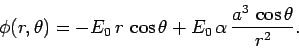 |
(836) |
Likewise, the most general solution inside the sphere, which satisfies
the boundary condition at , is
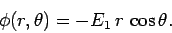 |
(837) |
The continuity of at yields
 |
(838) |
Likewise, the matching condition (835) gives
 |
(839) |
Hence,
Note that the electric field inside the sphere is uniform, parallel
to the external electric field outside the sphere, and of magnitude  . Moreover,
  , provided that
  . Finally,
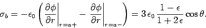
the density of the bound charge sheet on the surface of the sphere
is
. Finally,
the density of the bound charge sheet on the surface of the sphere
is
 |
(842) |
As a final example, consider a spherical cavity, of radius , in a
uniform dielectric medium, of dielectric constant , in the presence of a
-directed electric field of magnitude . This problem is analogous
to the previous problem, except that the matching condition
(835) becomes
 |
(843) |
Hence,
Note that the field inside the cavity is uniform, parallel
to the external electric field outside the sphere, and of magnitude . Moreover,  , provided that . The density
of the bound charge sheet on the surface of the cavity
is
, provided that . The density
of the bound charge sheet on the surface of the cavity
is
 |
(846) |
Next: Energy density within a
Up: Dielectric and magnetic media
Previous: Boundary conditions for and
Richard Fitzpatrick
2006-02-02