


Next: Complex analysis
Up: Electrostatics
Previous: One-dimensional solution of Poisson's
The method of images
Suppose that we have a point charge  held a distance
  from an infinite,
grounded, conducting plate. Let the plate lie in the
from an infinite,
grounded, conducting plate. Let the plate lie in the  -
- plane, and suppose that
the point charge is located at coordinates (0, 0, ). What is the
scalar potential above the plane? This is not a simple question because the point
charge induces surface charges on the plate, and we do not know how these
are distributed.
plane, and suppose that
the point charge is located at coordinates (0, 0, ). What is the
scalar potential above the plane? This is not a simple question because the point
charge induces surface charges on the plate, and we do not know how these
are distributed.
What do we know in this problem? We know that the conducting plate is an
equipotential surface. In fact, the potential of the plate is zero, since it is grounded.
We also know that the potential at infinity is zero (this is our usual boundary
condition for the scalar potential). Thus, we need to solve Poisson's equation
in the region  , for a single point charge at position (0, 0, ),
subject to the boundary conditions
, for a single point charge at position (0, 0, ),
subject to the boundary conditions
 |
(710) |
and
 |
(711) |
as
 . Let us forget about the real problem, for a
moment, and concentrate on a slightly different one. We refer to this as the
analogue problem. In the analogue problem, we have a charge located at
(0, 0, ) and a charge
. Let us forget about the real problem, for a
moment, and concentrate on a slightly different one. We refer to this as the
analogue problem. In the analogue problem, we have a charge located at
(0, 0, ) and a charge  located at (0, 0, -), with no conductors present.
We can easily find the scalar potential for this problem, since we know where
all the charges are located. We get
located at (0, 0, -), with no conductors present.
We can easily find the scalar potential for this problem, since we know where
all the charges are located. We get
 |
(712) |
Note, however, that
 |
(713) |
and
 |
(714) |
as
. In addition,
 satisfies Poisson's equation
for a charge at (0, 0, ), in the region . Thus,
is a solution
to the problem posed earlier, in the region . Now, the uniqueness theorem tells
us that there is only one solution to Poisson's equation
which satisfies a given, well-posed set of boundary conditions. So,
must be the correct potential in the region .
Of course,
is completely wrong in the region
satisfies Poisson's equation
for a charge at (0, 0, ), in the region . Thus,
is a solution
to the problem posed earlier, in the region . Now, the uniqueness theorem tells
us that there is only one solution to Poisson's equation
which satisfies a given, well-posed set of boundary conditions. So,
must be the correct potential in the region .
Of course,
is completely wrong in the region  .
We know this because the grounded plate shields the region from the
point charge, so that
.
We know this because the grounded plate shields the region from the
point charge, so that  in this region. Note that we are leaning pretty
heavily on the uniqueness theorem here! Without this theorem,
it would be hard to convince
a skeptical person that
in this region. Note that we are leaning pretty
heavily on the uniqueness theorem here! Without this theorem,
it would be hard to convince
a skeptical person that
 is the correct solution
in the region .
is the correct solution
in the region .
Now that we know the potential in the region , we can easily work
out the distribution of charges induced on the conducting plate. We already
know that the relation between the electric
field immediately above a conducting surface
and the density of charge on the surface is
 |
(715) |
In this case,
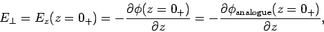 |
(716) |
so
 |
(717) |
It follows from Eq. (712) that
![\begin{displaymath}
\frac{\partial\phi}{\partial z} = \frac{q}{4\pi \epsilon_0...
...-d)^2]^{3/2}} +
\frac{(z+d)}{[x^2+y^2+(z+d)^2]^{3/2}}\right\},
\end{displaymath}](img1499.png) |
(718) |
so
 |
(719) |
Clearly, the charge induced on the plate has the opposite sign to the point charge.
The charge density on the plate is also symmetric about the  -axis, and is largest
where the plate is closest to the point charge. The total charge induced on the
plate is
-axis, and is largest
where the plate is closest to the point charge. The total charge induced on the
plate is
 |
(720) |
which yields
 |
(721) |
where  . Thus,
![\begin{displaymath}
Q = - \frac{q d}{2} \int_0^\infty \frac{dk}{(k+d^2)^{3/2}}
= q d\left[ \frac{1}{(k+d^2)^{1/2}}\right]_0^\infty = - q.
\end{displaymath}](img1504.png) |
(722) |
So, the total charge induced on the plate is equal and opposite to the point charge
which induces it.
Our point charge induces charges of the opposite sign on the conducting plate.
This, presumably, gives rise to a force of attraction between the charge and the
plate. What is this force? Well, since the potential, and, hence, the electric
field, in the vicinity of the point charge is the same as in the analogue problem,
then the force on the charge must be the same as well. In the analogue problem,
there are two charges  a net distance
  apart. The force on
the charge at position (0, 0, ) (i.e., the real charge) is
apart. The force on
the charge at position (0, 0, ) (i.e., the real charge) is
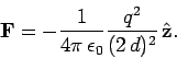 |
(723) |
What, finally, is the potential energy of the system. For the analogue problem
this is just
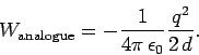 |
(724) |
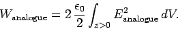
Note that the fields on opposite sides of the conducting plate are mirror images
of one another in the analogue problem. So are the charges (apart from the change
in sign). This is why the technique of replacing conducting surfaces by
imaginary charges is called the method of images. We know that the potential
energy
of a set of charges is equivalent to the energy stored in the electric field.
Thus,
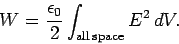 |
(725) |
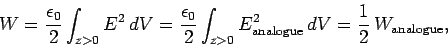
In the analogue problem, the fields on either side of the - plane are
mirror images of one another, so
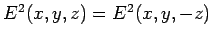 . It follows
that
. It follows
that
 |
(726) |
In the real problem
So,
 |
(729) |
giving
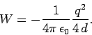 |
(730) |
There is another method by which we can obtain the above result. Suppose that
the charge is gradually moved towards the plate along the -axis from infinity
until it reaches position (0, 0, ). How much work is required to
achieve this? We know that the force of attraction acting on the charge is
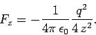 |
(731) |
Thus, the work required to move this charge by  is
is
 |
(732) |
The total work needed to move the charge from  to
to  is
is
![\begin{displaymath}
W = \frac{1}{4\pi \epsilon_0}\int_{\infty}^d \frac{q^2}{4\...
...t]_{\infty}^d
= - \frac{1}{4\pi \epsilon_0} \frac{q^2}{4 d}.
\end{displaymath}](img1520.png) |
(733) |
Of course, this work is equivalent to the potential energy we evaluated earlier,
and is, in turn, the same as the energy contained in the electric field.
As a second example of the method of images, consider a grounded spherical conductor
of radius  placed at the origin. Suppose that a charge is
placed outside the sphere at
placed at the origin. Suppose that a charge is
placed outside the sphere at  , where
  . What is
the force of attraction between the sphere and the charge? In this case,
we proceed by considering an analogue problem in which the sphere is replaced by an image charge
. What is
the force of attraction between the sphere and the charge? In this case,
we proceed by considering an analogue problem in which the sphere is replaced by an image charge  placed
somewhere on the -axis at
placed
somewhere on the -axis at  . The electric potential throughout space in the
analogue problem is simply
. The electric potential throughout space in the
analogue problem is simply
![\begin{displaymath}
\phi = \frac{q}{4\pi \epsilon_0} \frac{1}{[(x-b)^2+y^2+z^2...
...\frac{q'}{4\pi \epsilon_0}
\frac{1}{[(x-c)^2+y^2+z^2]^{1/2}}.
\end{displaymath}](img1525.png) |
(734) |
The image charge is chosen so as to make the surface correspond to
the surface of the sphere. Setting the above expresion to zero, and performing
a little algebra, we find that the surface satisfies
 |
(735) |
where
 . Of course, the surface of the sphere satisfies
 |
(736) |
The above two equations can be made identical by setting  and
and
 ,
or
,
or
 |
(737) |
and
 |
(738) |
According to the uniqueness theorem, the potential in the analogue problem is
now identical with that in the real problem, outside the sphere. (Of course, in the real
problem, the potential inside the sphere is zero.)
Hence, the
force of attraction between the sphere and the original charge in the real problem
is the same as the force of attraction between the two charges in the analogue
problem. It follows that
 |
(739) |
There are many other image problems, each of which involves replacing a conductor
with an imaginary charge (or charges) which mimics the electric
field in some region (but not everywhere). Unfortunately, we do not
have time to discuss any more of these problems.
Next: Complex analysis
Up: Electrostatics
Previous: One-dimensional solution of Poisson's
Richard Fitzpatrick
2006-02-02