Next: Relativity and electromagnetism
Up: Electromagnetic radiation
Previous: Reflection at a dielectric
A wave-guide is a hollow conducting pipe, of uniform cross-section, used to transport high frequency
electromagnetic waves (generally, in the microwave band) from one
point to another. The main advantage of wave-guides is their relatively
low level of radiation losses (since the electric and
magnetic fields are completely enclosed by a conducting wall) compared to transmission lines.
Consider a vacuum-filled wave-guide which runs parallel to the  -axis.
An electromagnetic wave trapped inside the wave-guide satisfies Maxwell's equations for free space:
-axis.
An electromagnetic wave trapped inside the wave-guide satisfies Maxwell's equations for free space:
 |
 |
 |
(1280) |
 |
|
|
(1281) |
 |
|
 |
(1282) |
 |
|
 |
(1283) |
Let
 , and
, and
 , where
  is the wave frequency, and
  the wave-number parallel to the axis of the wave-guide.
It follows that
the wave-number parallel to the axis of the wave-guide.
It follows that
 |
|
|
(1284) |
 |
|
|
(1285) |
 |
|
 |
(1286) |
 |
|
 |
(1287) |
 |
|
 |
(1288) |
 |
|
 |
(1289) |
 |
|
 |
(1290) |
 |
|
 |
(1291) |
Equations (1287) and (1289) yield
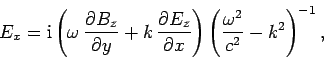 |
(1292) |
and
 |
(1293) |
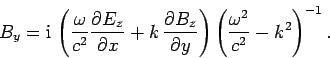
Likewise, Eqs. (1286) and (1290) yield
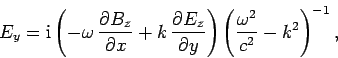 |
(1294) |
and
 |
(1295) |
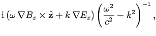
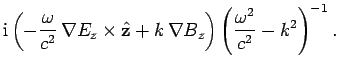
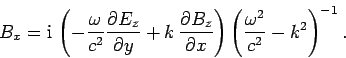
These equations can be combined to give
Here,  and
and  are the transverse electric
and magnetic fields: i.e., the electric and
magnetic fields in the
are the transverse electric
and magnetic fields: i.e., the electric and
magnetic fields in the  -
- plane. It is clear, from Eqs. (1296) and (1297), that the transverse fields are fully determined once the
longitudinal fields,
plane. It is clear, from Eqs. (1296) and (1297), that the transverse fields are fully determined once the
longitudinal fields,  and
and  , are known.
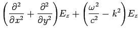
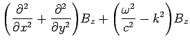
Substitution of Eqs. (1296) and (1297) into Eqs. (1288) and (1291) yields the equations satisfied by
the longitudinal fields:
The remaining equations, (1284) and (1285), are automatically
satisfied provided Eqs. (1296)-(1299) are satisfied.
We expect
 inside the walls of the wave-guide,
assuming that they are perfectly conducting. Hence, the appropriate
boundary conditions at the walls are
inside the walls of the wave-guide,
assuming that they are perfectly conducting. Hence, the appropriate
boundary conditions at the walls are
It follows, by inspection of Eqs. (1296) and (1297), that
these boundary conditions are satisfied provided
at the walls. Here,  is the normal vector to the walls.
Hence, the electromagnetic fields inside the wave-guide are fully
specified by solving Eqs. (1298) and (1299), subject to
the boundary conditions (1302) and (1303), respectively.
is the normal vector to the walls.
Hence, the electromagnetic fields inside the wave-guide are fully
specified by solving Eqs. (1298) and (1299), subject to
the boundary conditions (1302) and (1303), respectively.
Equations (1298) and (1299) support two independent types
of solution. The first type has  , and is consequently called a transverse electric, or TE, mode. Conversely, the
second type has
, and is consequently called a transverse electric, or TE, mode. Conversely, the
second type has  , and is called a transverse
magnetic, or TM, mode.
, and is called a transverse
magnetic, or TM, mode.
Consider the specific example of a rectangular wave-guide, with conducting walls
at  , and
, and  . For a TE mode, the longitudinal
magnetic field can be written
. For a TE mode, the longitudinal
magnetic field can be written
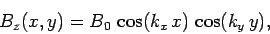 |
(1304) |
The boundary condition (1303) requires that
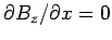 at , and
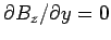 at . It follows that
where
 , and
, and
 . Clearly, there are
many different kinds of TE mode, corresponding to the many different
choices of
. Clearly, there are
many different kinds of TE mode, corresponding to the many different
choices of  and
and  . Let us refer to a mode corresponding to
a particular choice of
. Let us refer to a mode corresponding to
a particular choice of  as a
as a  mode. Note, however, that there
is no
mode. Note, however, that there
is no  mode, since
  is uniform in this case.
According to
Eq. (1299), the dispersion relation for the mode is
given by
is uniform in this case.
According to
Eq. (1299), the dispersion relation for the mode is
given by
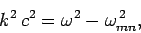 |
(1307) |
where
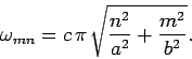 |
(1308) |
According to the dispersion relation (1307), is imaginary for
 . In other words, for
wave frequencies below
. In other words, for
wave frequencies below  , the mode
fails to propagate down the wave-guide, and is instead attenuated. Hence,
is termed the cut-off frequency for the mode.
Assuming that
, the mode
fails to propagate down the wave-guide, and is instead attenuated. Hence,
is termed the cut-off frequency for the mode.
Assuming that  , the TE mode with the lowest cut-off frequency is
the
, the TE mode with the lowest cut-off frequency is
the  mode, where
 |
(1309) |
For frequencies above the cut-off frequency, the phase-velocity of the
mode is given by
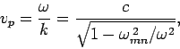 |
(1310) |
which is greater than  . However, the group-velocity takes the form
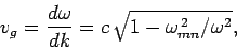 |
(1311) |
which is always less than . Of course, energy is transmitted down the wave-guide
at the group-velocity, rather than the phase-velocity. Note that the group-velocity goes to zero as the
wave frequency approaches the cut-off frequency.
For a TM mode, the longitudinal electric field can be written
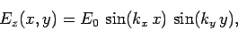 |
(1312) |
The boundary condition (1302) requires that
at , and . It follows that
where
 , and
, and
 . The dispersion relation
for the
. The dispersion relation
for the  mode is also given by Eq. (1307).
Hence, Eqs. (1310) and (1311) also apply to TM modes.
However, the TM mode with the lowest cut-off frequency is the
mode is also given by Eq. (1307).
Hence, Eqs. (1310) and (1311) also apply to TM modes.
However, the TM mode with the lowest cut-off frequency is the
 mode, where
 |
(1315) |
It follows that the mode with the lowest cut-off frequency is always
a TE mode.
There is, in principle, a third type of mode which can propagate down
a wave-guide. This third mode type is characterized by  ,
and is consequently called a transverse electromagnetic, or
TEM, mode. It is easily seen, from an inspection of
Eqs. (1286)-(1291), that a TEM mode satisfies
,
and is consequently called a transverse electromagnetic, or
TEM, mode. It is easily seen, from an inspection of
Eqs. (1286)-(1291), that a TEM mode satisfies
 |
(1316) |
and
where  satisfies
 |
(1319) |
The boundary conditions (1302) and (1303) imply
that
 |
(1320) |
at the walls. However, there is no non-trivial solution of Eqs. (1319)
and (1320) for a conventional wave-guide. In other words,
conventional wave-guides do not support TEM modes.
In fact, it turns out that only wave-guides with central conductors
support TEM modes. Consider, for instance, a co-axial wave-guide
in which the electric and magnetic fields are trapped between two
parallel concentric cylindrical conductors of radius  and
and  (with
(with  ).
In this case,
).
In this case,  , and Eq. (1319) reduces to
 |
(1321) |
where  is a standard cylindrical polar coordinate.
The boundary condition (1320) is automatically satisfied at
is a standard cylindrical polar coordinate.
The boundary condition (1320) is automatically satisfied at  and
and
 .
The above equation has the following non-trivial solution:
.
The above equation has the following non-trivial solution:
 |
(1322) |
Note, however, that the inner conductor must be present, otherwise
 as
as
 , which is unphysical.
According to the dispersion relation (1316), TEM modes have
no cut-off frequency, and have the phase-velocity (and group-velocity) .
Indeed, this type of mode is the same as that supported by a transmission line
(see Sect. 7.7).
, which is unphysical.
According to the dispersion relation (1316), TEM modes have
no cut-off frequency, and have the phase-velocity (and group-velocity) .
Indeed, this type of mode is the same as that supported by a transmission line
(see Sect. 7.7).
Next: Relativity and electromagnetism
Up: Electromagnetic radiation
Previous: Reflection at a dielectric
Richard Fitzpatrick
2006-02-02