Secular evolution of planetary orbits
As a specific example of the use of orbital perturbation theory,
let us determine the evolution of the osculating orbital elements of the two planets in our model solar system
due to the secular terms in their disturbing functions (i.e., the terms that are independent of the
mean longitudes
 and
and
 ). This is equivalent to averaging the osculating
elements over the relatively short timescales associated with the periodic terms in the disturbing functions
(i.e., the terms that depend on
and
, and, therefore, oscillate on timescales similar
to the orbital periods of the planets).
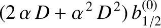
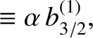
From Equations (10.16)–(10.18),
the secular part of the first planet's disturbing function takes the form
). This is equivalent to averaging the osculating
elements over the relatively short timescales associated with the periodic terms in the disturbing functions
(i.e., the terms that depend on
and
, and, therefore, oscillate on timescales similar
to the orbital periods of the planets).
From Equations (10.16)–(10.18),
the secular part of the first planet's disturbing function takes the form
 |
(10.29) |
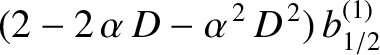
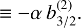
where
because, as can be demonstrated (Brouwer and Clemence 1961),
Evaluating the right-hand sides of Equations (10.10)–(10.15)
to
 (it is assumed that
  ,
,
 ,
,  ,
,  ,
,  ,
,  ,
,  ,
,  ,
,  ,
,  ,
,  ), we find that
 |
 |
(10.34) |
 |
 |
(10.35) |
 |
 |
(10.36) |
 |
 |
(10.37) |
 |
 |
(10.38) |
 |
 |
(10.39) |
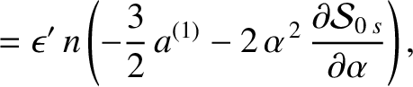
 . It follows that
  , and
, and
 |
![$\displaystyle =\skew{5}\bar{\lambda}_0+ n\left[1-\epsilon'\,\alpha^{\,2}\,D\,b_{1/2}^{(0)}\right] t,$](img2523.png) |
(10.40) |
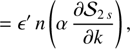
|
![$\displaystyle = \epsilon'\,n\left[\frac{1}{4}\,k\,\alpha^{\,2}\,b^{(1)}_{3/2}-\frac{1}{4}\,k'\,\alpha^{\,2}\,b_{3/2}^{(2)}\right],$](img2524.png) |
(10.41) |
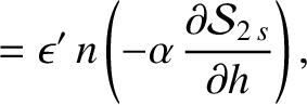
|
![$\displaystyle = \epsilon'\,n\left[ -\frac{1}{4}\,h\,\alpha^{\,2}\,b^{(1)}_{3/2}+\frac{1}{4}\,h'\,\alpha^{\,2}\,b_{3/2}^{(2)}\right],$](img2525.png) |
(10.42) |
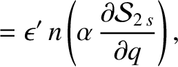
|
![$\displaystyle = \epsilon'\,n\left[ -\frac{1}{4}\,q\,\alpha^{\,2}\,b^{(1)}_{3/2}+\frac{1}{4}\,q'\,\alpha^{\,2}\,b_{3/2}^{(1)}\right],$](img2526.png) |
(10.43) |
|
![$\displaystyle = \epsilon'\,n\left[ \frac{1}{4}\,p\,\alpha^{\,2}\,b^{(1)}_{3/2}-\frac{1}{4}\,p'\,\alpha^{\,2}\,b_{3/2}^{(1)}\right].$](img2527.png) |
(10.44) |
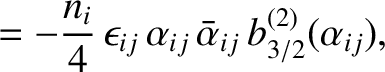
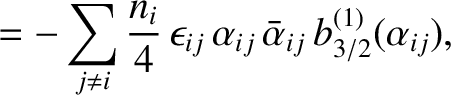
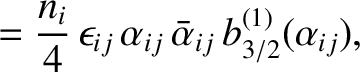
From Equations (10.26)–(10.28),
the secular part of the second planet's disturbing function takes the form
 |
(10.45) |
where
Evaluating the right-hand sides of Equations (10.20)–(10.25)
to
 , we find that
 |
|
(10.48) |
 |
 |
(10.49) |
 |
 |
(10.50) |
 |
 |
(10.51) |
 |
 |
(10.52) |
 |
 |
(10.53) |
 , and
, and
 |
![$\displaystyle =\skew{5}\bar{\lambda}_0'+n'\left[1-\epsilon\,D\left(\alpha\,b_{1/2}^{(0)}\right)\right] t,$](img2542.png) |
(10.54) |
|
![$\displaystyle = \epsilon \,n'\left[\frac{1}{4}\,k'\,\alpha\,b^{(1)}_{3/2}-\frac{1}{4}\,k\,\alpha\,b_{3/2}^{(2)}\right],$](img2543.png) |
(10.55) |
|
![$\displaystyle = \epsilon\,n' \left[-\frac{1}{4}\,h'\,\alpha\,b^{(1)}_{3/2}+\frac{1}{4}\,h\,\alpha\,b_{3/2}^{(2)}\right],$](img2544.png) |
(10.56) |
|
![$\displaystyle = \epsilon \,n'\left[-\frac{1}{4}\,q'\,\alpha\,b^{(1)}_{3/2}+\frac{1}{4}\,q\,\alpha\,b_{3/2}^{(1)}\right],$](img2545.png) |
(10.57) |
|
![$\displaystyle = \epsilon\,n'\left[\frac{1}{4}\,p'\,\alpha\,b^{(1)}_{3/2}-\frac{1}{4}\,p\,\alpha\,b_{3/2}^{(1)}\right].$](img2546.png) |
(10.58) |
Let us now generalize the preceding analysis to take all eight of the major planets in the solar system into account.
Let planet  (where runs from
  to
to  ) have mass
  , major radius
  , eccentricity
  , longitude of the
perihelion
, longitude of the
perihelion  , inclination
  , and longitude of the ascending node
 .
As before, it is convenient to introduce the alternative orbital elements
.
As before, it is convenient to introduce the alternative orbital elements
 ,
,
 ,
,
 , and
, and
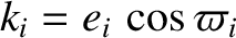
 . It is also helpful to define the following parameters:
![\begin{displaymath}\alpha_{ij} =\left\{
\begin{array}{ccc}
a_i/a_j&\mbox{\hspace{1cm}}&a_j>a_i\\ [0.5ex]
a_j/a_i&&a_j<a_i
\end{array}\right.,\end{displaymath}](img2556.png) |
(10.59) |
and
![\begin{displaymath}\bar{\alpha}_{ij} =\left\{
\begin{array}{ccc}
a_i/a_j&\mbox{\hspace{1cm}}&a_j>a_i\\ [0.5ex]
1&&a_j<a_i
\end{array}\right.,\end{displaymath}](img2557.png) |
(10.60) |
as well as
where  is the mass of the Sun.
It then follows, from the preceding analysis, that the secular terms in the planetary disturbing functions cause the
is the mass of the Sun.
It then follows, from the preceding analysis, that the secular terms in the planetary disturbing functions cause the
 ,
,  ,
,  , and
, and  to vary in time as
where
to vary in time as
where
 |
 |
(10.67) |
 |
 |
(10.68) |
 |
 |
(10.69) |
 |
 |
(10.70) |
 .
Here, Mercury is planet 1, Venus is planet 2, and so on, and Neptune is planet 8. Note that the
time evolution of the and the , which determine the eccentricities of the planetary orbits, is decoupled from that of the and the , which determine the inclinations.
Let us search for normal mode
solutions to Equations (10.63)–(10.66) of the form
It follows that
At this stage, we have effectively reduced the problem of determining the secular evolution of the planetary orbits to a pair of matrix eigenvalue equations (Gradshteyn and Ryzhik 1980c)
that can be solved via standard numerical techniques (Press et al. 1992). Once we have determined the eigenfrequencies,
.
Here, Mercury is planet 1, Venus is planet 2, and so on, and Neptune is planet 8. Note that the
time evolution of the and the , which determine the eccentricities of the planetary orbits, is decoupled from that of the and the , which determine the inclinations.
Let us search for normal mode
solutions to Equations (10.63)–(10.66) of the form
It follows that
At this stage, we have effectively reduced the problem of determining the secular evolution of the planetary orbits to a pair of matrix eigenvalue equations (Gradshteyn and Ryzhik 1980c)
that can be solved via standard numerical techniques (Press et al. 1992). Once we have determined the eigenfrequencies,  and
and  ,
and the corresponding eigenvectors,
,
and the corresponding eigenvectors,  and
and  , we can find the phase angles
  and
and  by demanding that, at
  , Equations (10.71)–(10.74) lead to the values of , , , and
given in Table 4.1.
, Equations (10.71)–(10.74) lead to the values of , , , and
given in Table 4.1.
Table 10.1:
Eigenfrequencies and phase angles obtained from Laplace-Lagrange secular evolution theory.
| |
|
|
|
|
 |
 |
 |
 |
 |
| |
|
|
|
|
| 1 |
5.462 |
-5.201 |
89.65 |
20.23 |
| 2 |
7.346 |
-6.570 |
195.0 |
318.3 |
| 3 |
17.33 |
-18.74 |
336.1 |
255.6 |
| 4 |
18.00 |
-17.64 |
319.0 |
296.9 |
| 5 |
3.724 |
0.000 |
30.12 |
107.5 |
| 6 |
22.44 |
-25.90 |
131.0 |
127.3 |
| 7 |
2.708 |
-2.911 |
109.9 |
315.6 |
| 8 |
0.6345 |
-0.6788 |
67.98 |
202.8 |
|
The theory outlined here is generally referred to as Laplace-Lagrange secular evolution theory. The
eigenfrequencies, eigenvectors, and phase angles obtained from this theory are listed in Tables 10.1–10.3.
Note that the largest eigenfrequency is of magnitude  arc seconds per year, which translates to an
oscillation period of about
arc seconds per year, which translates to an
oscillation period of about
 years. In other words, the typical timescale over which the secular evolution of the solar system predicted by Laplace-Lagrange theory takes place is at least
years, and is, therefore, much
longer than the orbital period of any planet.
years. In other words, the typical timescale over which the secular evolution of the solar system predicted by Laplace-Lagrange theory takes place is at least
years, and is, therefore, much
longer than the orbital period of any planet.
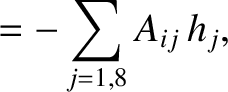
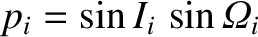
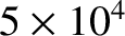
Figure: 10.2
The full circles show the observed planetary perihelion precession rates (left-hand panel) and ascending node
precession rates (right-hand panel) at J2000. All ascending nodes are measured relative to the mean ecliptic at J2000. The empty circles show the theoretical
precession rates calculated from Laplace-Lagrange secular evolution theory.
Source (for observational data): Standish and Williams (1992).
|
|
Figure 10.2 compares the observed perihelion and ascending node precession rates of the planets at (which
corresponds to the epoch J2000) with those calculated from the theory described previously. It can be seen that, generally, there
is good agreement between the theoretical and observed precession rates, which gives us some degree of confidence in the
theory. On the whole, the degree of agreement exhibited in the left-hand panel of Figure 10.2 is
better than that exhibited in Figure 5.1, indicating that the Laplace-Lagrange secular evolution theory
described in this chapter is an improvement on the (highly simplified) Gaussian secular evolution theory
outlined in Section 5.4.
Observe that one of the inclination eigenfrequencies,  , takes the value zero. This is a consequence of the conservation
of angular momentum. Because the solar system is effectively an isolated dynamical system, its net angular momentum
vector,
, takes the value zero. This is a consequence of the conservation
of angular momentum. Because the solar system is effectively an isolated dynamical system, its net angular momentum
vector,  , is constant in both magnitude and direction. The plane normal to that passes through the
center of mass of the solar system (which lies very close to the Sun) is known as the invariable plane. If all
of the planetary orbits were to lie in the invariable plane then the net angular velocity vector of the solar system would be
parallel to its fixed net angular momentum vector. Moreover, the angular momentum vector would be parallel to one of
the solar system's principal axes of rotation. In this situation, we would expect the solar system to remain in
the invariable plane. (See Chapter 8.) In other words, we would not expect any time evolution of the planetary
inclinations. (Of course, lack of time variation implies an eigenfrequency of zero.) According to Equations (10.73) and (10.74), and the
data shown in Tables 10.1 and 10.3, if the solar system were in the inclination eigenstate associated with
the null eigenfrequency, , then we would have
, is constant in both magnitude and direction. The plane normal to that passes through the
center of mass of the solar system (which lies very close to the Sun) is known as the invariable plane. If all
of the planetary orbits were to lie in the invariable plane then the net angular velocity vector of the solar system would be
parallel to its fixed net angular momentum vector. Moreover, the angular momentum vector would be parallel to one of
the solar system's principal axes of rotation. In this situation, we would expect the solar system to remain in
the invariable plane. (See Chapter 8.) In other words, we would not expect any time evolution of the planetary
inclinations. (Of course, lack of time variation implies an eigenfrequency of zero.) According to Equations (10.73) and (10.74), and the
data shown in Tables 10.1 and 10.3, if the solar system were in the inclination eigenstate associated with
the null eigenfrequency, , then we would have
for 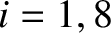 .
Because
and
, it follows that all of the
planetary orbits would lie in the same plane, and this plane—which is, of course, the invariable plane—is
inclined at
.
Because
and
, it follows that all of the
planetary orbits would lie in the same plane, and this plane—which is, of course, the invariable plane—is
inclined at
 to the ecliptic plane. Furthermore, the
longitude of the ascending node of the invariable plane,
with respect to the ecliptic plane, is
to the ecliptic plane. Furthermore, the
longitude of the ascending node of the invariable plane,
with respect to the ecliptic plane, is
 . Actually, it is generally more convenient to measure
the inclinations of the planetary orbits with respect to the invariable plane, rather than the ecliptic plane, because the
inclination of the latter plane varies in time. We can achieve this goal by simply omitting the fifth inclination
eigenstate when calculating orbital inclinations from Equations (10.73) and (10.74).
. Actually, it is generally more convenient to measure
the inclinations of the planetary orbits with respect to the invariable plane, rather than the ecliptic plane, because the
inclination of the latter plane varies in time. We can achieve this goal by simply omitting the fifth inclination
eigenstate when calculating orbital inclinations from Equations (10.73) and (10.74).
-8pt
Table: 10.2
Components of eccentricity eigenvectors obtained from Laplace-Lagrange secular evolution theory.
All components multiplied by  .
.
| |
|
|
|
|
|
|
|
|
| |
 |
2 |
3 |
4 |
5 |
6 |
7 |
8 |
| |
|
|
|
|
|
|
|
|
 |
18128 |
629 |
404 |
66 |
0 |
0 |
0 |
0 |
| 2 |
-2331 |
1919 |
1497 |
265 |
-1 |
-1 |
0 |
0 |
| 3 |
154 |
-1262 |
1046 |
2979 |
0 |
0 |
0 |
0 |
| 4 |
-169 |
1489 |
-1485 |
7281 |
0 |
0 |
0 |
0 |
| 5 |
2446 |
1636 |
1634 |
1878 |
4331 |
3416 |
-4388 |
159 |
| 6 |
10 |
-51 |
242 |
1562 |
-1560 |
4830 |
-180 |
-13 |
| 7 |
59 |
58 |
62 |
82 |
207 |
189 |
2999 |
-322 |
| 8 |
0 |
1 |
1 |
2 |
6 |
6 |
144 |
954 |
|
Consider the th planet. Suppose one of the coefficients— , say—is sufficiently large that
 |
(10.79) |
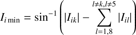
This is known as the Lagrange condition (Hagihara 1971). As can be demonstrated, if the Lagrange condition is satisfied then the eccentricity of the
th planet's orbit varies between the minimum value
 |
(10.80) |
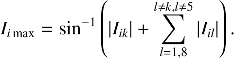
and the maximum value
 |
(10.81) |
Moreover, on average, the th planet's perihelion point precesses at the associated eigenfrequency,  . The precession
is prograde (i.e., in the same direction as the orbital motion) if the frequency is positive,
and retrograde (i.e., in the opposite direction) if the frequency is negative.
If the Lagrange condition is not satisfied then all we can say is that the maximum eccentricity is given by Equation (10.81),
and there is no minimum eccentricity (i.e., the eccentricity can vary all the way down to zero). Furthermore,
no mean precession rate of the perihelion point can be identified.
It can be seen from Table 10.2 that the Lagrange condition for the orbital eccentricities is satisfied for all planets except
for Venus and Earth. The maximum and minimum eccentricities, and mean perihelion precession rates, of the
planets (when they exist) are given in Table 10.4. Note that Jupiter and Uranus have the same mean
perihelion precession rates, and that all planets that possess mean precession rates exhibit prograde precession.
. The precession
is prograde (i.e., in the same direction as the orbital motion) if the frequency is positive,
and retrograde (i.e., in the opposite direction) if the frequency is negative.
If the Lagrange condition is not satisfied then all we can say is that the maximum eccentricity is given by Equation (10.81),
and there is no minimum eccentricity (i.e., the eccentricity can vary all the way down to zero). Furthermore,
no mean precession rate of the perihelion point can be identified.
It can be seen from Table 10.2 that the Lagrange condition for the orbital eccentricities is satisfied for all planets except
for Venus and Earth. The maximum and minimum eccentricities, and mean perihelion precession rates, of the
planets (when they exist) are given in Table 10.4. Note that Jupiter and Uranus have the same mean
perihelion precession rates, and that all planets that possess mean precession rates exhibit prograde precession.
Table: 10.3
Components of inclination eigenvectors obtained from Laplace-Lagrange secular evolution theory.
All components multiplied by .
| |
|
|
|
|
|
|
|
|
| |
|
2 |
3 |
4 |
5 |
6 |
7 |
8 |
| |
|
|
|
|
|
|
|
|
|
12548 |
1180 |
850 |
180 |
-2 |
-2 |
2 |
0 |
| 2 |
-3548 |
1006 |
811 |
180 |
-1 |
-1 |
0 |
0 |
| 3 |
409 |
-2684 |
2446 |
-3595 |
0 |
0 |
0 |
0 |
| 4 |
116 |
-685 |
451 |
5021 |
0 |
-1 |
0 |
0 |
| 5 |
2751 |
2751 |
2751 |
2751 |
2751 |
2751 |
2751 |
2751 |
| 6 |
27 |
14 |
279 |
954 |
-636 |
1587 |
-69 |
-7 |
| 7 |
-333 |
-191 |
-173 |
-125 |
-95 |
-77 |
1757 |
-206 |
| 8 |
-144 |
-132 |
-129 |
-122 |
-116 |
-112 |
109 |
1181 |
|
There is also a Lagrange condition associated with the inclinations of the planetary orbits (Hagihara 1971).
This condition is satisfied for the th planet if one of the — , say—is sufficiently large that
 |
(10.82) |
The fifth inclination eigenmode is omitted from this summation because we are now
measuring inclinations relative to the invariable plane.
If the Lagrange condition is satisfied then the inclination of the
th planet's orbit with respect to the invariable plane varies between the minimum value
 |
(10.83) |
and the maximum value
 |
(10.84) |
Moreover, on average, the ascending node precesses at the associated eigenfrequency,  . The precession
is prograde (i.e., in the same direction as the orbital motion) if the frequency is positive,
and retrograde (i.e., in the opposite direction) if the frequency is negative.
If the Lagrange condition is not satisfied then all we can say is that the maximum inclination is given by Equation (10.84),
and there is no minimum inclination (i.e., the inclination can vary all the way down to zero). Furthermore,
no mean precession rate of the ascending node can be identified.
It can be seen from Table 10.3 that the Lagrange condition for the orbital inclinations is satisfied for all planets except
for Venus, Earth, and Mars. The maximum and minimum inclinations, and mean nodal precession rates, of the
planets (when they exist) are given in Table 10.4. The four outer planets, which
possess most of the mass of the solar system, all have orbits whose inclinations to the invariable plane remain small.
On the other hand, the four relatively light inner planets have orbits whose inclinations to the invariable
plane can become relatively large. Observe that Jupiter and Saturn have the same mean
nodal precession rates, and that all planets that possess mean precession rates exhibit retrograde precession.
. The precession
is prograde (i.e., in the same direction as the orbital motion) if the frequency is positive,
and retrograde (i.e., in the opposite direction) if the frequency is negative.
If the Lagrange condition is not satisfied then all we can say is that the maximum inclination is given by Equation (10.84),
and there is no minimum inclination (i.e., the inclination can vary all the way down to zero). Furthermore,
no mean precession rate of the ascending node can be identified.
It can be seen from Table 10.3 that the Lagrange condition for the orbital inclinations is satisfied for all planets except
for Venus, Earth, and Mars. The maximum and minimum inclinations, and mean nodal precession rates, of the
planets (when they exist) are given in Table 10.4. The four outer planets, which
possess most of the mass of the solar system, all have orbits whose inclinations to the invariable plane remain small.
On the other hand, the four relatively light inner planets have orbits whose inclinations to the invariable
plane can become relatively large. Observe that Jupiter and Saturn have the same mean
nodal precession rates, and that all planets that possess mean precession rates exhibit retrograde precession.
Table 10.4:
Maximum/minimum eccentricities and inclinations of planetary orbits, and mean perihelion/nodal precession rates,
from Laplace-Lagrange secular evolution theory. All inclinations relative to invariable plane.
| |
|
|
|
|
|
|
| Planet |
 |
 |
 |
 |
 |
 |
| |
|
|
|
|
|
|
| Mercury |
0.130 |
0.233 |
 |
4.57 |
9.86 |
 |
| Venus |
0.000 |
0.0705 |
 |
0.000 |
3.38 |
|
| Earth |
0.000 |
0.0638 |
|
0.000 |
2.95 |
|
| Mars |
0.0444 |
0.141 |
 |
0.000 |
5.84 |
|
| Jupiter |
0.0256 |
0.0611 |
 |
0.241 |
0.489 |
 |
| Saturn |
0.0121 |
0.0845 |
 |
0.797 |
1.02 |
|
| Uranus |
0.0106 |
0.0771 |
|
0.902 |
1.11 |
 |
| Neptune |
0.00460 |
0.0145 |
 |
0.554 |
0.800 |
 |
|
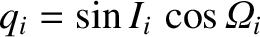
Figure 10.3:
Time variation of the eccentricity (top left), inclination (top right), perihelion precession
rate (bottom left), and ascending node precession rate (bottom right), of Mercury, as predicted by Laplace-Lagrange
secular perturbation theory. Time is measured in millions of years relative to J2000. All inclinations
are relative to the invariable plane. The horizontal dashed lines in the top panels
indicate the predicted minimum and maximum eccentricities and inclinations from
Table 10.4. The horizontal dashed lines in the bottom panels
indicate the predicted mean perihelion and ascending node precession rates from same
table.
|
|
Figure 10.3 shows the time variation of the eccentricity, inclination, perihelion precession
rate, and ascending node precession rate, of Mercury, as predicted by the Laplace-Lagrange
secular perturbation theory described earlier. It can be seen that the eccentricity and inclination
do indeed oscillate between the upper and lower bounds specified in Table 10.4.
Moreover, the perihelion and ascending node precession rates do appear to oscillate about the mean values ( and ,
respectively) specified in the same table.
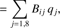
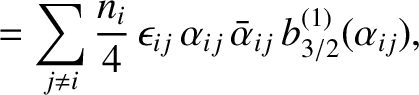
Figure 10.4:
The eccentricity eigenfrequencies obtained from Brouwer and van Woerkom's
refinement of standard Laplace-Lagrange secular evolution theory (filled circles), compared with the corresponding
eigenfrequencies from Table 10.1 (open circles).
|
|
According to Laplace-Lagrange secular perturbation theory, the mutual gravitational interactions between the various planets in the
solar system cause their orbital eccentricities and inclinations to oscillate between fixed bounds on
timescales that are long compared to their orbital periods. Recall, however, that these results depend on a great many approximations; the neglect of all nonsecular terms in the
planetary disturbing functions, as well as the neglect of secular terms beyond first order in the planetary masses, and
beyond second order in the orbital eccentricities and inclinations. It turns out that, when the neglected
terms are included in the analysis, the largest correction
to standard Laplace-Lagrange theory is a second-order (in the planetary masses) effect caused by periodic
terms in the disturbing functions of Jupiter and Saturn that oscillate on a relatively long timescale (i.e., almost 900 years), due to
the fact that the orbital periods of these two planets are almost commensurable (i.e., five times the orbital period of
Jupiter is almost equal to two times the orbital period of Saturn). In 1950, Brouwer and van Woerkom worked out a modified version of Laplace-Lagrange
secular perturbation theory that takes the aforementioned correction into account (Brouwer and van Woerkom 1950). This refined secular evolution theory is
described, in detail, in Murray and Dermott (1999). As is illustrated in Figure 10.4, the values of the
eccentricity eigenfrequencies and
in the Brouwer–van Woerkom theory differ somewhat from those specified in Table 10.1. The
corresponding eigenvectors are also somewhat modified. The Brouwer–van Woerkom theory contains two additional, relatively small-amplitude, eccentricity eigenmodes that
oscillate at the eigenfrequencies
 and
and
 . On the other hand, the Brouwer–van Woerkom theory does not give rise to any significant modifications to the inclination eigenmodes.
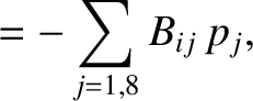
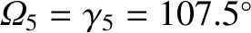
Figure 10.5 shows the maximum and minimum orbital eccentricities predicted by the Brouwer–van Woerkom
theory, compared with the corresponding limits from Table 10.4. It can be seen that the refinements introduced
by Brouwer and van Woerkom modify the oscillation limits for the orbital eccentricities of Mercury and Uranus somewhat, but do
not significantly change the limits for the other planets. Of course, the oscillation limits for the orbital inclinations are
unaffected by these refinements (because the inclination eigenmodes are unaffected).
. On the other hand, the Brouwer–van Woerkom theory does not give rise to any significant modifications to the inclination eigenmodes.
Figure 10.5 shows the maximum and minimum orbital eccentricities predicted by the Brouwer–van Woerkom
theory, compared with the corresponding limits from Table 10.4. It can be seen that the refinements introduced
by Brouwer and van Woerkom modify the oscillation limits for the orbital eccentricities of Mercury and Uranus somewhat, but do
not significantly change the limits for the other planets. Of course, the oscillation limits for the orbital inclinations are
unaffected by these refinements (because the inclination eigenmodes are unaffected).
Figure 10.5:
The maximum and minimum orbital eccentricities predicted by Brouwer and van Woerkom's
refinement of standard Laplace-Lagrange secular evolution theory (filled circles), compared with the corresponding
limits from Table 10.4 (open circles).
|
|
It must be emphasized that the Brouwer–van Woerkom secular evolution theory is only approximate in nature. In fact,
the theory is capable of predicting the secular
evolution of the solar system with reasonable accuracy up to a million or so years into the future or the past.
However, over longer timescales, it becomes inaccurate because the true long-term dynamics
of the solar system contains chaotic elements. These elements originate from two secular resonances among the
planet:
 , which is related to the gravitational interaction of Mars and the Earth; and
 , which is related to the interaction of Mercury, Venus, and Jupiter (Laskar 1990).


![$\displaystyle = [G\,(M+m_i)/a_i^{\,3}]^{1/2},$](img2561.png)

![\includegraphics[height=2.75in]{Chapter09/fig9_02.eps}](img2599.png)


![\includegraphics[height=5.5in]{Chapter09/fig9_03.eps}](img2632.png)
![\includegraphics[height=3.25in]{Chapter09/fig9_04.eps}](img2633.png)
![\includegraphics[height=3.25in]{Chapter09/fig9_05.eps}](img2636.png)