Next: Generalized momenta Up: Lagrangian mechanics Previous: Generalized forces
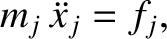
 , where
 are each equal to the mass of the
first particle,
are each equal to the mass of the
first particle,
 are each equal to the mass of the
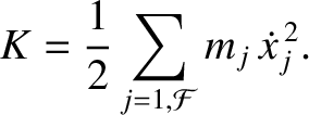
second particle, and so forth. Furthermore, the kinetic energy of the
system can be written
are each equal to the mass of the
second particle, and so forth. Furthermore, the kinetic energy of the
system can be written
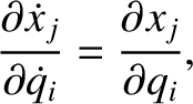
Because
 , we can write
 |
(7.11) |
.
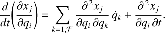
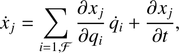
Hence, it follows that
 . According to the
preceding equation,
where we are treating the
. According to the
preceding equation,
where we are treating the
 and the
  as independent
variables.
as independent
variables.
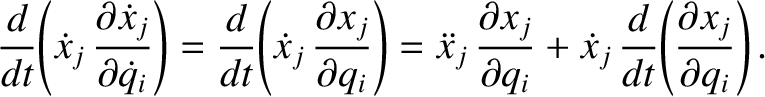
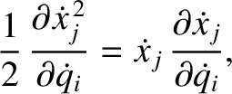
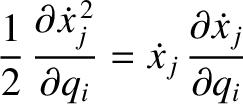
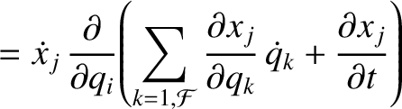
Multiplying Equation (7.12) by
 , and then differentiating
with respect to time, we obtain
, and then differentiating
with respect to time, we obtain
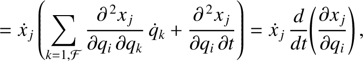
Let us take Equation (7.17), multiply by  , and then sum over all
  .
We obtain
.
We obtain
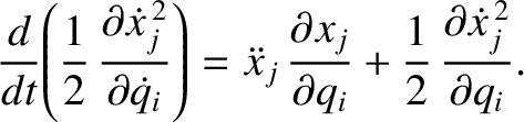
 |
(7.18) |
 |
(7.19) |
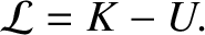
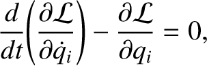
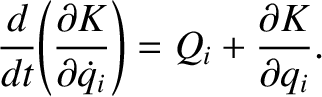
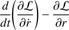
It is helpful to introduce a function  , called the Lagrangian, that
is defined as the difference between the kinetic and potential energies of the dynamical system under investigation:
, called the Lagrangian, that
is defined as the difference between the kinetic and potential energies of the dynamical system under investigation:
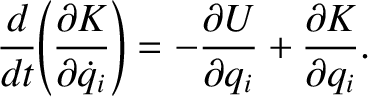
 is clearly independent of the
, it follows from Equation (7.20) that
for
is clearly independent of the
, it follows from Equation (7.20) that
for
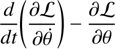
 . This equation is known as Lagrange's equation.
According to the preceding analysis, if we can express the kinetic and potential energies of our dynamical system solely in terms of our generalized coordinates and their time derivatives then we can immediately write down the equations of motion of the system, expressed in terms of the generalized coordinates, using Lagrange's equation, Equation (7.22). Unfortunately, this scheme only works for conservative systems.
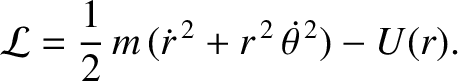
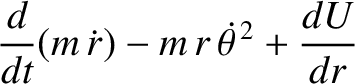
As an example, consider a particle of mass  moving in two dimensions in the central potential
  . This is clearly a two-degree-of-freedom dynamical system.
As described in Section 4.4, the particle's instantaneous position
is most conveniently specified in terms of the plane polar
coordinates
. This is clearly a two-degree-of-freedom dynamical system.
As described in Section 4.4, the particle's instantaneous position
is most conveniently specified in terms of the plane polar
coordinates  and
and  . These are our two generalized coordinates.
According to Equation (4.13), the square of the particle's velocity
can be written
. These are our two generalized coordinates.
According to Equation (4.13), the square of the particle's velocity
can be written
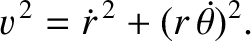 |
(7.23) |
 |
 |
 |
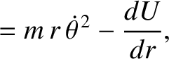 |
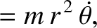
(7.25) |
 |
 |
 |
 |
(7.26) |
 |
 |
(7.27) |
 |
|
(7.28) |
 |
|
(7.29) |
 |
|
(7.30) |
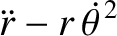
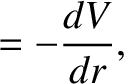
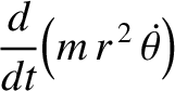
 , and
, and  is a constant. We recognize Equations (7.31) and (7.32) as the equations
that we derived in Chapter 4 for motion in a central potential.
The advantage of the Lagrangian method of deriving these equations is
that we avoid having to express the acceleration in terms of the generalized
coordinates and .
is a constant. We recognize Equations (7.31) and (7.32) as the equations
that we derived in Chapter 4 for motion in a central potential.
The advantage of the Lagrangian method of deriving these equations is
that we avoid having to express the acceleration in terms of the generalized
coordinates and .