Next: Potential due to uniform Up: Newtonian gravity Previous: Gravitational potential energy
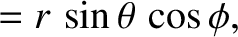
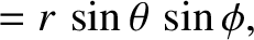
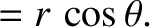
 , aligned along the
  -axis. These coordinates are related to
regular Cartesian coordinates as follows (see Section A.8):
-axis. These coordinates are related to
regular Cartesian coordinates as follows (see Section A.8):
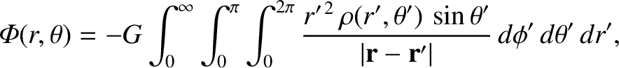
Consider an axially symmetric mass distribution; that is, a
 that is independent of the azimuthal angle,
  . We would expect
such a mass distribution to generated an axially symmetric gravitational
potential,
. We would expect
such a mass distribution to generated an axially symmetric gravitational
potential,
 . Hence, without loss of generality, we can
set
. Hence, without loss of generality, we can
set  when evaluating
 from Equation (3.10). In fact,
given that
from Equation (3.10). In fact,
given that
 in spherical coordinates, this equation yields
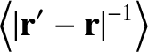
. However, because
 is independent of
  , Equation (3.27)
can also be written
where
, Equation (3.27)
can also be written
where
 denotes an average over the azimuthal angle.
Now,
 |
(3.29) |
 |
(3.30) |
)
 |
(3.31) |
 |
(3.32) |
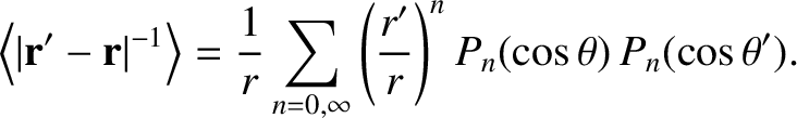
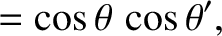
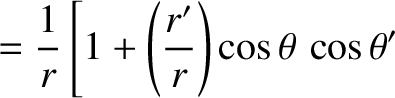
Suppose that  . In this case, we can expand
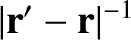 as a convergent power series in
  , to give
![$\displaystyle \vert{\bf r}'-{\bf r}\vert^{-1}= \frac{1}{r}\left[
1 + \left(\fra...
...rac{r'}{r}\right)^2(3\,F^{\,2}-1)
+ {\cal O}\left(\frac{r'}{r}\right)^3\right].$](img404.png) |
(3.33) |
. Because
 ,
,
 , and
, and
 , it is easily seen that
 |
 |
(3.34) |
 |
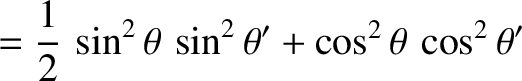 |
|
 |
(3.35) |
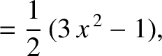
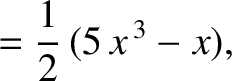
Now, the well-known Legendre polynomials,  , are defined (Abramowitz and Stegun 1965b) as
![$\displaystyle P_n(x) = \frac{1}{2^n\,n!}\,\frac{d^{\,n}}{dx^{\,n}}\!\left[(x^{\,2}-1)^n\right],$](img417.png) |
(3.37) |
 .
It follows that
and so on.
The Legendre polynomials are mutually
orthogonal:
(Abramowitz and Stegun 1965b).
Here,
.
It follows that
and so on.
The Legendre polynomials are mutually
orthogonal:
(Abramowitz and Stegun 1965b).
Here,
 is 1 if
  , and 0 otherwise. The Legendre polynomials also form a complete set; any function
of
, and 0 otherwise. The Legendre polynomials also form a complete set; any function
of  that is well behaved in the interval
 can be represented as a weighted sum of the . Likewise,
any function of
can be represented as a weighted sum of the . Likewise,
any function of  that is well behaved in the interval
 can
be represented as a weighted
sum of the
can
be represented as a weighted
sum of the
 .
.
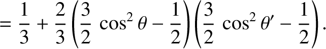
A comparison of Equation (3.36) and Equations (3.38)–(3.40) makes it reasonably clear that, when , the complete expansion
of
 is
is
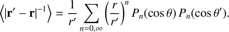
 , we can expand in powers of
  to obtain
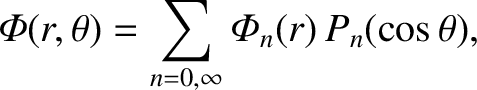
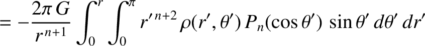
It follows from Equations (3.28), (3.43), and (3.44)
that
where
to obtain
It follows from Equations (3.28), (3.43), and (3.44)
that
where
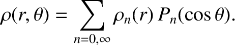
Given that the
form a complete set, we can always
write
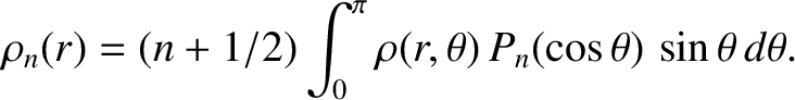 |
(3.48) |
,
generated by an axially symmetric mass distribution,
 .
.


![$\displaystyle \phantom{=}+\left.\left(\frac{r'}{r}\right)^2\left(\frac{3}{2}\co...
...}\cos^2\theta'-\frac{1}{2}\right)
+ {\cal O}\left(\frac{r'}{r}\right)^3\right].$](img415.png)