


Next: Exercises
Up: Spin Angular Momentum
Previous: Factorization of Spinor-Wavefunctions
Spin Greater Than One-Half Systems
We have seen how to deal with a spin-half particle in quantum mechanics.
But, what happens if we have a spin one or a spin three-halves particle?
It turns out that we can generalize the Pauli two-component scheme in a fairly
straightforward manner. Consider a spin- particle: that is, a particle for which
the eigenvalue of
particle: that is, a particle for which
the eigenvalue of  is
is
 . Here,
is either an integer, or a half-integer. The eigenvalues of
. Here,
is either an integer, or a half-integer. The eigenvalues of  are written
 , where
 is allowed to take the values
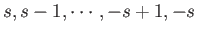 . In fact,
there are
. In fact,
there are  distinct allowed values of
. Not surprisingly, we can represent
the state of the particle by
different wavefunctions, denoted
distinct allowed values of
. Not surprisingly, we can represent
the state of the particle by
different wavefunctions, denoted
 . Here,
specifies the probability density
for observing the particle at position
. Here,
specifies the probability density
for observing the particle at position  with spin angular
momentum
in the
with spin angular
momentum
in the  -direction. More exactly,
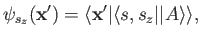 |
(5.111) |
where
 denotes a state ket in the product of the position
and spin spaces. The state of the particle can be represented more
succinctly by a spinor-wavefunction,
denotes a state ket in the product of the position
and spin spaces. The state of the particle can be represented more
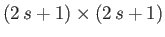
succinctly by a spinor-wavefunction,  , which is simply the
component column
vector of the
.
Thus, a spin one-half particle is represented by a two-component spinor-wavefunction,
a spin one particle by a three-component spinor-wavefunction, a spin three-halves particle
by a four-component spinor-wavefunction, and so on.
, which is simply the
component column
vector of the
.
Thus, a spin one-half particle is represented by a two-component spinor-wavefunction,
a spin one particle by a three-component spinor-wavefunction, a spin three-halves particle
by a four-component spinor-wavefunction, and so on.
In this extended Schrödinger/Pauli
scheme, position space operators take the form of diagonal
 matrix differential operators. Thus, we can represent the momentum operators
as
matrix differential operators. Thus, we can represent the momentum operators
as
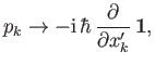 |
(5.112) |
where  is the
unit matrix. [See
Equation (5.91).]
We represent the spin
operators as
is the
unit matrix. [See
Equation (5.91).]
We represent the spin
operators as
 |
(5.113) |
where the
extended Pauli matrix  (which is, of course, Hermitian) has elements
 |
(5.114) |
Here,  ,
,  are integers, or half-integers, lying in the range
  to
to  .
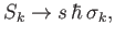
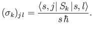
But, how can we evaluate the brackets
.
But, how can we evaluate the brackets
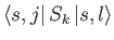 and, thereby, construct the extended Pauli matrices? In fact, it is trivial
to construct the
and, thereby, construct the extended Pauli matrices? In fact, it is trivial
to construct the  matrix. By definition,
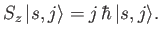 |
(5.115) |
Hence,
 |
(5.116) |
where use has been made of the orthonormality property of the
 .
Thus,
is the suitably normalized diagonal matrix of the eigenvalues
of
. The elements of
.
Thus,
is the suitably normalized diagonal matrix of the eigenvalues
of
. The elements of  and
and  are most easily
obtained by considering the ladder operators,
are most easily
obtained by considering the ladder operators,
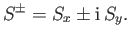 |
(5.117) |
We know, from Equations (4.55)-(4.56), that
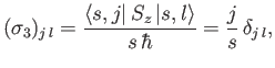
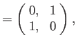
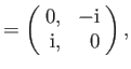
It follows from Equations (5.114), and (5.117)-(5.119), that
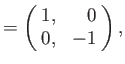
According to Equations (5.116) and (5.120)-(5.121), the Pauli matrices for a spin one-half
( )
particle (e.g., an electron, a proton, or a neutron) are
)
particle (e.g., an electron, a proton, or a neutron) are
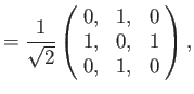
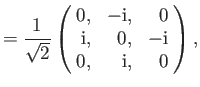
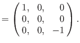
as we have seen previously. For a spin one ( ) particle (e.g., a
  -boson or a
  -boson), we find that
In fact, we can now construct the Pauli matrices for a particle of arbitrary spin.
This means that we can convert the general energy eigenvalue problem for a spin-
particle, where the Hamiltonian is some function of position and spin operators,
into
coupled partial differential equations involving the
wavefunctions
 . Unfortunately, such a system
of equations is generally too complicated
to solve exactly.
. Unfortunately, such a system
of equations is generally too complicated
to solve exactly.
Next: Exercises
Up: Spin Angular Momentum
Previous: Factorization of Spinor-Wavefunctions
Richard Fitzpatrick
2016-01-22
![$\displaystyle = \frac{[s\,(s+1) - j\,(j-1)]^{1/2} }{2\,s}\,\delta_{j\,\, l+1}+ \frac{[s\,(s+1) - j\,(j+1)]^{1/2} }{2\,s}\,\delta_{j\,\, l-1},$](img1556.png)
![$\displaystyle = \frac{[ s\,(s+1) - j\,(j-1)]^{1/2} }{2\,{\rm i}\,s}\,\delta_{j\,\, l+1}- \frac{[s\,(s+1) - j\,(j+1)]^{1/2} }{2\,{\rm i}\,s}\,\delta_{j\,\, l-1}.$](img1558.png)