Next: Schrödinger Representation
Up: Position and Momentum
Previous: Poisson Brackets
Consider a simple system with one classical degree of freedom, which corresponds to
the Cartesian coordinate  . Suppose that
is free to take any value (e.g.,
could be the position of a free particle). The classical dynamical variable
is represented in quantum
mechanics as a linear Hermitian operator that is also called
.
Moreover, the operator
possesses eigenvalues
. Suppose that
is free to take any value (e.g.,
could be the position of a free particle). The classical dynamical variable
is represented in quantum
mechanics as a linear Hermitian operator that is also called
.
Moreover, the operator
possesses eigenvalues  lying in the continuous
range
lying in the continuous
range
 (because the eigenvalues
correspond to all the possible results of a measurement of
). We can
span ket space using the suitably normalized eigenkets of
.
An eigenket corresponding to the eigenvalue
is denoted
(because the eigenvalues
correspond to all the possible results of a measurement of
). We can
span ket space using the suitably normalized eigenkets of
.
An eigenket corresponding to the eigenvalue
is denoted
 .
Moreover,
.
Moreover,
 |
(2.26) |
[See Equation (1.88).]
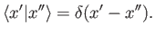
The eigenkets satisfy the extremely useful relation
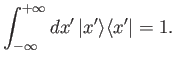 |
(2.27) |
[See Equation (1.94).]
This formula expresses the fact that the eigenkets are complete, mutually
orthogonal, and suitably normalized.
A state ket  (which represents a general state
  of the system)
can be expressed as a linear superposition of the eigenkets of the position
operator using Equation (2.27). Thus,
of the system)
can be expressed as a linear superposition of the eigenkets of the position
operator using Equation (2.27). Thus,
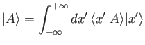 |
(2.28) |
The quantity
 is a complex function of the position eigenvalue
. We can write
is a complex function of the position eigenvalue
. We can write
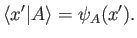 |
(2.29) |
Here,
 is the famous wavefunction of quantum mechanics [99,32].
Note that state
is completely specified by its wavefunction
[because the wavefunction can be used to reconstruct the state ket
using Equation (2.28)].
It is clear that the wavefunction of state
is simply the collection
of the weights of the corresponding state ket
,
when it is expanded in terms of the eigenkets of the
position operator. Recall, from Section 1.10, that the probability of
a measurement of a dynamical variable
is the famous wavefunction of quantum mechanics [99,32].
Note that state
is completely specified by its wavefunction
[because the wavefunction can be used to reconstruct the state ket
using Equation (2.28)].
It is clear that the wavefunction of state
is simply the collection
of the weights of the corresponding state ket
,
when it is expanded in terms of the eigenkets of the
position operator. Recall, from Section 1.10, that the probability of
a measurement of a dynamical variable  yielding the result
  when the system is in (a properly normalized) state
is given by
when the system is in (a properly normalized) state
is given by
 , assuming that
the
eigenvalues of
are discrete. This result is easily generalized to dynamical
variables possessing continuous eigenvalues. In fact, the probability of
a measurement of
yielding a result lying in the range
to
, assuming that
the
eigenvalues of
are discrete. This result is easily generalized to dynamical
variables possessing continuous eigenvalues. In fact, the probability of
a measurement of
yielding a result lying in the range
to  when the system is in a state
is
when the system is in a state
is
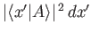 .
In other words, the probability of a measurement of position yielding a
result in the range
to
when the wavefunction of the system is
is
.
In other words, the probability of a measurement of position yielding a
result in the range
to
when the wavefunction of the system is
is
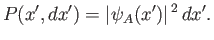 |
(2.30) |
This formula is only valid if the state ket
is properly normalized:
that is, if
 . The corresponding normalization for
the wavefunction is
. The corresponding normalization for
the wavefunction is
 |
(2.31) |
Consider a second state  represented by a state ket
  and
a wavefunction
and
a wavefunction
 . The inner product
 can be written
 |
(2.32) |
where use has been made of Equations (2.27) and (2.29). Thus, the inner product of two states is
related to the overlap integral of their wavefunctions.
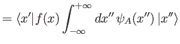
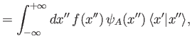
Consider a general function  of the observable
[e.g.,
of the observable
[e.g.,
 ].
If
].
If
 then it follows that
giving
 |
(2.34) |
where use has been made of Equation (2.26). (See Exercise 3.) Here,  is the same function
of the position eigenvalue
that
is of the position operator
.
For instance, if
then
is the same function
of the position eigenvalue
that
is of the position operator
.
For instance, if
then
 . It follows, from the previous result,
that a general state ket
can be written
. It follows, from the previous result,
that a general state ket
can be written
 |
(2.35) |
where  is the same function of the operator
that the wavefunction
is of the position eigenvalue
, and the ket
is the same function of the operator
that the wavefunction
is of the position eigenvalue
, and the ket  has the
wavefunction
has the
wavefunction
 . The ket
is termed the standard ket.
The dual of the standard ket is termed the standard bra, and is
denoted
. The ket
is termed the standard ket.
The dual of the standard ket is termed the standard bra, and is
denoted  . It is
easily seen that
. It is
easily seen that
 |
(2.36) |
Note, finally, that
 is often shortened to
 , leaving
the dependence on the position operator
tacitly understood.
, leaving
the dependence on the position operator
tacitly understood.
Next: Schrödinger Representation
Up: Position and Momentum
Previous: Poisson Brackets
Richard Fitzpatrick
2016-01-22