


Next: Simple Pendulum
Up: One-Dimensional Motion
Previous: Periodic Driving Forces
Transients
We saw, in Section 3.7, that when a one-dimensional dynamical system,
close to a stable equilibrium point, is subject to a sinusoidal external
force of the form (104) then the equation of motion of the
system is written
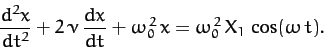 |
(132) |
We also found that the solution to this equation which oscillates in sympathy
with the applied force takes the form
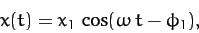 |
(133) |
where  and
and  are specified in Equations (110) and (111), respectively.
However, (133) is not the most general solution to Equation (132).
It should be clear that we can take the above solution and add to it
any solution of Equation (132) calculated with the right-hand side set to zero,
and the result will also be a solution of Equation (132).
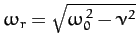
Now, we investigated the solutions to (132) with the right-hand
set to zero in Section 3.5. In the underdamped regime (
are specified in Equations (110) and (111), respectively.
However, (133) is not the most general solution to Equation (132).
It should be clear that we can take the above solution and add to it
any solution of Equation (132) calculated with the right-hand side set to zero,
and the result will also be a solution of Equation (132).
Now, we investigated the solutions to (132) with the right-hand
set to zero in Section 3.5. In the underdamped regime ( ),
we found that the most general such solution takes the
form
),
we found that the most general such solution takes the
form
 |
(134) |
where  and
and  are two arbitrary constants [they are in fact the integration constants
of the second-order ordinary differential equation (132)],
and
are two arbitrary constants [they are in fact the integration constants
of the second-order ordinary differential equation (132)],
and
 . Thus,
the most general solution to Equation (132) is written
. Thus,
the most general solution to Equation (132) is written
 |
(135) |
The first two terms on the right-hand side of the above equation
are called transients, since they decay in time. The transients
are determined by the initial conditions. However, if we wait
long enough after setting the system into motion then the transients will
always decay away, leaving the time-asymptotic solution (133), which is independent of the
initial conditions.
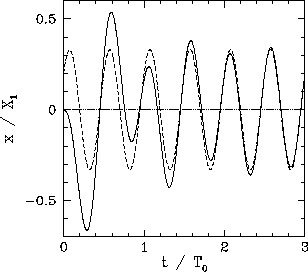
Figure 8:
Transients.
 |
As an example, suppose that we set the system into motion at time
 with the initial conditions
 .
Setting
.
Setting  in Equation (135), we obtain
 |
(136) |
Moreover, setting  in Equation (135), we get
 |
(137) |
Thus, we have now determined the constants and , and, hence,
fully specified the solution for  . Figure 8
shows this solution (solid curve) calculated for
. Figure 8
shows this solution (solid curve) calculated for
 and
and
 . Here,
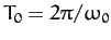 . The associated time-asymptotic solution (133)
is also shown for the sake of comparison (dashed curve). It can
be seen that the full solution quickly converges to the time-asymptotic
solution.
. The associated time-asymptotic solution (133)
is also shown for the sake of comparison (dashed curve). It can
be seen that the full solution quickly converges to the time-asymptotic
solution.
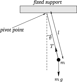
Figure 9:
A simple pendulum.
 |
Next: Simple Pendulum
Up: One-Dimensional Motion
Previous: Periodic Driving Forces
Richard Fitzpatrick
2011-03-31