


Next: Generalized Forces
Up: Lagrangian Dynamics
Previous: Introduction
Let the  , for
, for  , be a set of coordinates which uniquely
specifies the instantaneous configuration of some dynamical system.
Here, it is assumed that each of the can vary independently.
The might be Cartesian coordinates, or polar
coordinates, or angles, or some mixture of all three types of coordinate, and are, therefore,
termed generalized coordinates. A dynamical system whose
instantaneous configuration is fully specified by
, be a set of coordinates which uniquely
specifies the instantaneous configuration of some dynamical system.
Here, it is assumed that each of the can vary independently.
The might be Cartesian coordinates, or polar
coordinates, or angles, or some mixture of all three types of coordinate, and are, therefore,
termed generalized coordinates. A dynamical system whose
instantaneous configuration is fully specified by  independent
generalized coordinates is said to have degrees of freedom.
For instance, the instantaneous position of a particle moving freely
in three dimensions is completely specified by its three Cartesian
coordinates,
independent
generalized coordinates is said to have degrees of freedom.
For instance, the instantaneous position of a particle moving freely
in three dimensions is completely specified by its three Cartesian
coordinates,  ,
,  , and
, and  . Moreover, these coordinates are clearly
independent of one another.
Hence, a dynamical
system consisting of a single particle moving
freely in three dimensions has three degrees of freedom. If there are two freely moving
particles then the system has six degrees of freedom, and so on.
. Moreover, these coordinates are clearly
independent of one another.
Hence, a dynamical
system consisting of a single particle moving
freely in three dimensions has three degrees of freedom. If there are two freely moving
particles then the system has six degrees of freedom, and so on.
Suppose that we have a dynamical system consisting of  particles
moving freely in three dimensions. This is an
particles
moving freely in three dimensions. This is an
 degree of
freedom system whose instantaneous configuration can be specified
by Cartesian coordinates. Let us denote these coordinates the
degree of
freedom system whose instantaneous configuration can be specified
by Cartesian coordinates. Let us denote these coordinates the
 , for
, for  . Thus,
  are the Cartesian coordinates
of the first particle,
are the Cartesian coordinates
of the first particle,  the Cartesian coordinates
of the second particle, etc. Suppose that the instantaneous configuration of the system can also be specified by generalized
coordinates, which we shall denote the , for . Thus, the
might be the spherical coordinates of the particles.
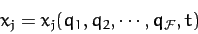
In general,
we expect the to be functions of the . In other words,
the Cartesian coordinates
of the second particle, etc. Suppose that the instantaneous configuration of the system can also be specified by generalized
coordinates, which we shall denote the , for . Thus, the
might be the spherical coordinates of the particles.
In general,
we expect the to be functions of the . In other words,
 |
(592) |
for . Here, for the sake of generality, we have included the
possibility that the functional relationship between the and the
might depend on the time,  , explicitly. This would be the
case if the dynamical system were subject to time varying constraints. For
instance, a system consisting of a particle constrained to move on a surface which is itself
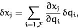
moving. Finally, by the chain rule, the variation of the due to a variation of the
(at constant ) is given by
, explicitly. This would be the
case if the dynamical system were subject to time varying constraints. For
instance, a system consisting of a particle constrained to move on a surface which is itself
moving. Finally, by the chain rule, the variation of the due to a variation of the
(at constant ) is given by
 |
(593) |
for .
Next: Generalized Forces
Up: Lagrangian Dynamics
Previous: Introduction
Richard Fitzpatrick
2011-03-31