Next: Zero-Velocity Surfaces
Up: The Three-Body Problem
Previous: Co-Rotating Frame
Let us search for possible equilibrium points of the mass  in the rotating reference frame. Such points
are termed Lagrange points. Thus, in the rotating frame, the mass would remain at rest if placed at one of the Lagrange points. It is, thus, clear that these points are
fixed in the rotating frame.
Conversely, in the inertial reference frame, the Lagrange points rotate about the center of mass with
angular velocity
in the rotating reference frame. Such points
are termed Lagrange points. Thus, in the rotating frame, the mass would remain at rest if placed at one of the Lagrange points. It is, thus, clear that these points are
fixed in the rotating frame.
Conversely, in the inertial reference frame, the Lagrange points rotate about the center of mass with
angular velocity  , and the mass would consequently also rotate about the center
of mass with angular velocity if placed at one of these points (with the appropriate
velocity). In the following,
we shall assumed, without loss of generality, that
, and the mass would consequently also rotate about the center
of mass with angular velocity if placed at one of these points (with the appropriate
velocity). In the following,
we shall assumed, without loss of generality, that  .
.
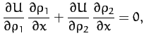
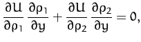
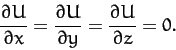
The Lagrange points satisfy
 in the rotating frame.
It thus follows, from Equations (1056)-(1058), that the Lagrange
points are the solutions of
in the rotating frame.
It thus follows, from Equations (1056)-(1058), that the Lagrange
points are the solutions of
 |
(1066) |
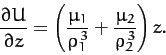
Now, it is easily seen that
 |
(1067) |
Since the term in brackets is positive definite, we conclude that the only solution to the
above equation is  . Hence, all of the Lagrange points lie in the
  -
- plane.
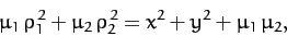
If then it is readily demonstrated that
 |
(1068) |
where use has been made of the fact that  .
Hence, Equation (1059) can also be written
.
Hence, Equation (1059) can also be written
 |
(1069) |
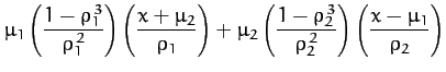
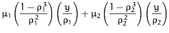
The Lagrange points thus satisfy
which reduce to
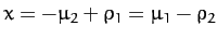
Now, one obvious solution of Equation (1073) is  , corresponding to a Lagrange
point which lies on the -axis. It turns out that there are three such points.
, corresponding to a Lagrange
point which lies on the -axis. It turns out that there are three such points.  lies between masses
  and
and  ,
,  lies to the right of mass , and
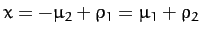
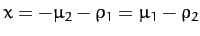
 lies to the left of mass --see Figure 48. At the point,
we have
lies to the left of mass --see Figure 48. At the point,
we have
 and
and
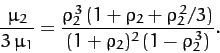
 . Hence, from Equation (1072),
 |
(1074) |
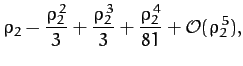
Assuming that  , we can find an approximate solution of Equation (1074)
by expanding in powers of
, we can find an approximate solution of Equation (1074)
by expanding in powers of  :
:
 |
(1075) |
This equation can be inverted to give
 |
(1076) |
where
 |
(1077) |
is assumed to be a small parameter.
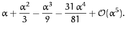
At the point,
we have
 and
and
 .
Hence, from Equation (1072),
.
Hence, from Equation (1072),
 |
(1078) |
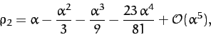
Again, expanding in powers of , we obtain
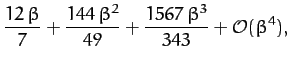
Finally, at the point,
we have
 and
and
 . Hence, from Equation (1072),
 |
(1081) |
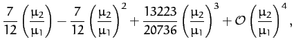
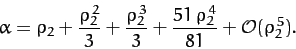
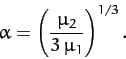
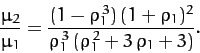
Let
 . Expanding in powers of
  , we obtain
where  is assumed to be a small parameter.
Let us now search for Lagrange points which do not lie on the -axis. One obvious solution of Equations (1070)
and (1071) is
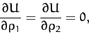 |
(1084) |
giving, from Equation (1069),
 |
(1085) |
or
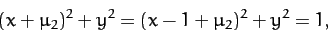 |
(1086) |
since 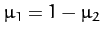 .
The two solutions of the above equation are
.
The two solutions of the above equation are
and specify the positions of the Lagrange points designated  and
and  . Note that point and the masses
and lie at the apexes of an equilateral triangle. The same is
true for point . We have now found all of the possible Lagrange points.
. Note that point and the masses
and lie at the apexes of an equilateral triangle. The same is
true for point . We have now found all of the possible Lagrange points.
Figure 49:
The masses and , and the five Lagrange points, to , calculated
for  .
.
 |
Figure 49 shows the positions of the two masses, and , and
the five Lagrange points, to , calculated for the case where .
Next: Zero-Velocity Surfaces
Up: The Three-Body Problem
Previous: Co-Rotating Frame
Richard Fitzpatrick
2011-03-31