Simple Pendulum

Consider a compact mass $m$ suspended from a light inextensible string of length $l$, such that the mass is free to swing from side to side in a vertical plane, as shown in Figure 9. This setup is known as a simple pendulum. Let $\theta$ be the angle subtended between the string and the downward vertical. Obviously, the stable equilibrium state of the simple pendulum corresponds to the situation in which the mass is stationary, and hangs vertically down (i.e., $\theta=0$). From elementary mechanics, the angular equation of motion of the pendulum is

$$I\,\frac{d^2{\theta}}{dt^2} = \tau,$$ (138)

where $I$ is the moment of inertia of the mass (see Section 8.3), and $\tau$ is the torque acting about the pivot point (see Section A.7). For the case in hand, given that the mass is essentially a point particle, and is situated a distance $l$ from the axis of rotation (i.e., the pivot point), it is easily seen that $I=m\,l^2$.

The two forces acting on the mass are the downward gravitational force, $m\,g$, where $g$ is the acceleration due to gravity, and the tension, $T$, in the string. Note, however, that the tension makes no contribution to the torque, since its line of action clearly passes through the pivot point. From simple trigonometry, the line of action of the gravitational force passes a distance $l\,\sin\theta$ from the pivot point. Hence, the magnitude of the gravitational torque is $m\,g\,l\, \sin\theta$. Moreover, the gravitational torque is a restoring torque: i.e., if the mass is displaced slightly from its equilibrium state (i.e., $\theta=0$) then the gravitational torque clearly acts to push the mass back toward that state. Thus, we can write

$$\tau = - m\,g\,l\,\sin\theta.$$ (139)

Combining the previous two equations, we obtain the following angular equation of motion of the pendulum:

$$l\,\frac{d^2{\theta}}{dt^2} +g\,\sin\theta=0.$$ (140)

Note that, unlike all of the other equations of motion which we have examined in this chapter, the above equation is nonlinear [since $\sin(a\,\theta)\neq a\,\sin\theta$, except when $\theta\ll 1$].

Let us assume, as usual, that the system does not stray very far from its equilibrium state ($\theta=0$). If this is the case then we can make the small angle approximation $\sin\theta\simeq \theta$, and the above equation of motion simplifies to

$$\frac{d^2\theta}{dt^2} + \omega_0^{\,2}\,\theta\simeq 0,$$ (141)

where $\omega_0 = \sqrt{g/l}$. Of course, this is just the simple harmonic equation. Hence, we can immediately write the solution as

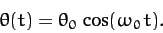$$\theta(t) = \theta_0\,\cos(\omega_0\,t).$$ (142)

We conclude that the pendulum swings back and forth at a fixed frequency, $\omega_0$, which depends on $l$ and $g$, but is independent of the amplitude, $\theta_0$, of the motion.

Suppose, now, that we desire a more accurate solution of Equation (140). One way in which we could achieve this would be to include more terms in the small angle expansion of $\sin\theta$, which is

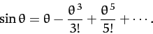$$\sin\theta = \theta - \frac{\theta^{\,3}}{3!} + \frac{\theta^{\,5}}{5!} +\cdots.$$ (143)

For instance, keeping the first two terms in this expansion, Equation (140) becomes

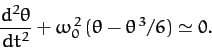$$\frac{d^2\theta}{dt^2} + \omega_0^{\,2}\,(\theta-\theta^{\,3}/6)\simeq 0.$$ (144)

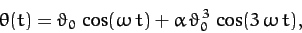
By analogy with (142), let us try a trial solution of the form

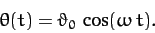$$\theta(t) = \vartheta_0\,\cos(\omega\,t).$$ (145)

Substituting this into Equation (144), and making use of the trigonometric identity

$$\cos^3 u \equiv (3/4)\,\cos u+ (1/4)\,\cos(3\,u),$$ (146)

we obtain

$$\vartheta_0\left[\omega_0^{\,2}-\omega^2 - (1/8)\,\omega_0^{... ...omega_0^{\,2}\,\vartheta_0^{\,3} \,\cos(3\,\omega\,t)\simeq 0.$$ (147)

It is evident that the above equation cannot be satisfied for all values of $t$, except in the trivial case $\vartheta_0=0$. However, the form of this expression does suggest a better trial solution, namely

$$\theta(t) = \vartheta_0\,\cos(\omega\,t) + \alpha\,\vartheta_0^{\,3}\,\cos(3\,\omega\,t),$$ (148)

where $\alpha$ is ${\cal O}(1)$. Substitution of this expression into Equation (144) yields

$$\vartheta_0\left[\omega_0^{\,2}-\omega^2 - (1/8)\,\omega_0^{\,2}\,\vartheta_0^{\,2} \right] \cos(\omega\,t) +$$

$$\vartheta_0^{\,3}\left[\alpha\,\omega_0^{\,2} - 9\,\alpha\,\omega^2- (1/24)\,\omega_0^{\,2}\right] \cos(3\,\omega\,t) + {\cal O}(\vartheta_0^{\,5}) \simeq 0.$$ (149)

We can only satisfy the above equation at all values of $t$, and for non-zero $\vartheta_0$, by setting the two expressions in square brackets to zero. This yields

$$\omega \simeq \omega_0 \,\sqrt{1-(1/8)\,\vartheta_0^{\,2}},$$ (150)

and

$$\alpha\simeq -\frac{\omega_0^{\,2}}{192}.$$ (151)

Now, the amplitude of the motion is given by

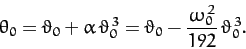$$\theta_0 = \vartheta_0 + \alpha\,\vartheta_0^{\,3} = \vartheta_0-\frac{\omega_0^{\,2}}{192}\,\vartheta_0^{\,3}.$$ (152)

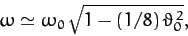
Hence, Equation (150) simplifies to

$$\omega = \omega_0\left[1-\frac{\theta_0^{\,2}}{16} + {\cal O}(\theta_0^{\,4})\right].$$ (153)

The above expression is only approximate, but it illustrates an important point: i.e., that the frequency of oscillation of a simple pendulum is not, in fact, amplitude independent. Indeed, the frequency goes down slightly as the amplitude increases.

The above example illustrates how we might go about solving a nonlinear equation of motion by means of an expansion in a small parameter (in this case, the amplitude of the motion).