Next: Potential Due to a
Up: Gravitational Potential Theory
Previous: Gravitational Potential
Axially Symmetric Mass Distributions
At this point, it is convenient to adopt standard spherical coordinates,
 , aligned along the
  -axis. These coordinates are related to
regular Cartesian coordinates as follows (see Section A.17):
-axis. These coordinates are related to
regular Cartesian coordinates as follows (see Section A.17):
Consider an axially symmetric mass distribution: i.e., a  which is independent of the azimuthal angle,
  . We would expect
such a mass distribution to generated an axially symmetric gravitational
potential,
. We would expect
such a mass distribution to generated an axially symmetric gravitational
potential,
 . Hence, without loss of generality, we can
set
. Hence, without loss of generality, we can
set  when evaluating
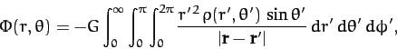
  from Equation (868). In fact,
given that
from Equation (868). In fact,
given that
 in spherical coordinates, this equation yields
 |
(872) |
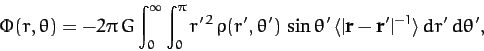
with the right-hand side evaluated at . However, since
 is independent of
  , the above equation
can also be written
, the above equation
can also be written
 |
(873) |
where
 denotes an average over the azimuthal angle,
.
denotes an average over the azimuthal angle,
.
Now,
 |
(874) |
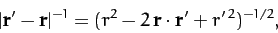
and
 |
(875) |
where (at )
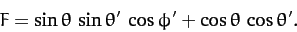 |
(876) |
Hence,
 |
(877) |
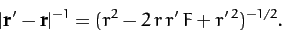
Suppose that  . In this case, we can expand
 as a convergent power series in
  , to give
![\begin{displaymath}
\vert{\bf r}'-{\bf r}\vert^{-1}= \frac{1}{r}\left[
1 + \left...
...ght)^2(3\,F^2-1)
+ {\cal O}\left(\frac{r'}{r}\right)^3\right].
\end{displaymath}](img2090.png) |
(878) |
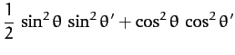
Let us now average this expression over the azimuthal angle, . Since
 ,
,
 , and
, and
 , it is easily seen that
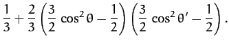
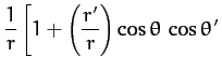
Hence,
Now, the well-known Legendre polynomials,  , are defined
![\begin{displaymath}
P_n(x) = \frac{1}{2^n\,n!}\,\frac{d^n}{dx^n}\!\left[(x^2-1)^n\right],
\end{displaymath}](img2103.png) |
(882) |
for  .
It follows that
.
It follows that
etc.
The Legendre polynomials are mutually
orthogonal: i.e.,
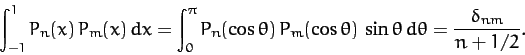 |
(886) |
Here,  is 1 if
  , and 0 otherwise. The Legendre polynomials also form a complete set: i.e., any well-behaved function
of
, and 0 otherwise. The Legendre polynomials also form a complete set: i.e., any well-behaved function
of  can be represented as a weighted sum of the . Likewise,
any well-behaved (even) function of
can be represented as a weighted sum of the . Likewise,
any well-behaved (even) function of  can be represented as a weighted
sum of the
can be represented as a weighted
sum of the
 .
.
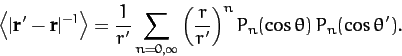
A comparison of Equation (881) and Equations (883)-(885) makes it reasonably clear that, when , the complete expansion
of
 is
is
 |
(887) |
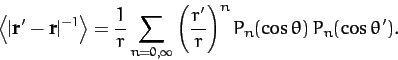
Similarly, when  , we can expand in powers of
  to obtain
 |
(888) |
It follows from Equations (873), (887), and (888)
that
 |
(889) |
where
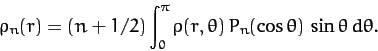
Now, given that the
form a complete set, we can always
write
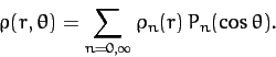 |
(891) |
This expression can be inverted, with the aid of Equation (886), to
give
 |
(892) |
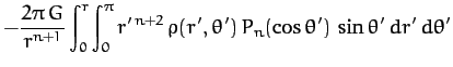
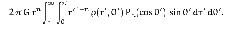
Hence, Equation (890) reduces to
 |
(893) |
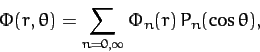
Thus, we now have a general expression for the gravitational potential,
,
generated by any axially symmetric mass distribution,
 .
.
Next: Potential Due to a
Up: Gravitational Potential Theory
Previous: Gravitational Potential
Richard Fitzpatrick
2011-03-31
![$\displaystyle +\left.\left(\frac{r'}{r}\right)^2\left(\frac{3}{2}\cos^2\theta-\...
...}\cos^2\theta'-\frac{1}{2}\right)
+ {\cal O}\left(\frac{r'}{r}\right)^3\right].$](img2101.png)