Gravitational Potential

Consider two point masses, $m$ and $m'$, located at position vectors ${\bf r}$ and ${\bf r}'$, respectively. According to Section 5.3, the acceleration ${\bf g}$ of mass $m$ due to the gravitational force exerted on it by mass $m'$ takes the form

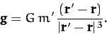$${\bf g} = G\,m'\,\frac{({\bf r}'-{\bf r})}{\vert{\bf r}'-{\bf r}\vert^{\,3}}.$$ (861)

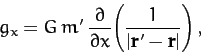
Now, the $x$-component of this acceleration is written

$$g_x = G\,m'\,\frac{(x'-x)}{[(x'-x)^2+(y'-y)^2+(z'-z)^2]^{\,3/2}},$$ (862)

where ${\bf r}=(x,\, y,\, z)$ and ${\bf r}' = (x',\,y',\,z')$. However, as is easily demonstrated,

$$\frac{(x'-x)}{[(x'-x)^2+(y'-y)^2+(z'-z)^2]^{\,3/2}}\equiv \frac{... ...tial}{\partial x}\!\left(\frac{1}{[(x'-x)^2+(y'-y)^2+(z'-z)^2]^{\,1/2}}\right).$$ (863)

Hence,

$$g_x = G\,m'\,\frac{\partial}{\partial x}\!\left(\frac{1}{\vert{\bf r}'-{\bf r}\vert}\right),$$ (864)

with analogous expressions for $g_y$ and $g_z$. It follows that

$${\bf g} = -\nabla\Phi,$$ (865)

where

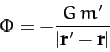$$\Phi = - \frac{G\,m'}{\vert{\bf r}'-{\bf r}\vert}$$ (866)

is termed the gravitational potential. Of course, we can only write ${\bf g}$ in the form (865) because gravity is a conservative force--see Chapter 2. Note that gravitational potential, $\Phi$, is directly related to gravitational potential energy, $U$. In fact, the potential energy of mass $m$ is $U=m\,\Phi$.

Now, it is well-known that gravity is a superposable force. In other words, the gravitational force exerted on some test mass by a collection of point masses is simply the sum of the forces exerted on the test mass by each point mass taken in isolation. It follows that the gravitational potential generated by a collection of point masses at a certain location in space is the sum of the potentials generated at that location by each point mass taken in isolation. Hence, using Equation (866), if there are $N$ point masses, $m_i$ (for $i=1, N$), located at position vectors ${\bf r}_i$, then the gravitational potential generated at position vector ${\bf r}$ is simply

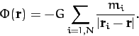$$\Phi({\bf r}) = - G\sum_{i=1,N} \frac{m_i}{\vert{\bf r}_i-{\bf r}\vert}.$$ (867)

Suppose, finally, that, instead of having a collection of point masses, we have a continuous mass distribution. In other words, let the mass at position vector ${\bf r}'$ be $\rho({\bf r}')\,d^3{\bf r}'$, where $\rho({\bf r}')$ is the local mass density, and $d^3{\bf r}'$ a volume element. Summing over all space, and taking the limit $d^3{\bf r}'\rightarrow 0$, Equation (867) yields

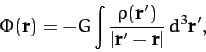$$\Phi({\bf r}) = - G\int\frac{\rho({\bf r}')}{\vert{\bf r}'-{\bf r}\vert}\,d^3{\bf r}',$$ (868)

where the integral is taken over all space. This is the general expression for the gravitational potential, $\Phi({\bf r})$, generated by a continuous mass distribution, $\rho({\bf r})$.