


Next: Uniform Flow
Up: Axisymmetric Incompressible Inviscid Flow
Previous: Axisymmetric Velocity Fields
In an irrotational flow pattern, we can automatically satisfy the constraint
 by writing
 |
(7.11) |
Suppose, however, that, in addition to being irrotational, the flow pattern is also incompressible: that is,
 . In
this case, Equation (7.11) yields
. In
this case, Equation (7.11) yields
 |
(7.12) |
In spherical coordinates, assuming that the flow pattern is axisymmetric, so that
 ,
the previous equation leads to (see Section C.4)
,
the previous equation leads to (see Section C.4)
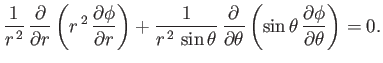 |
(7.13) |
Let us search for a separable solution of Equation (7.13) of the form
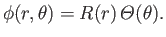 |
(7.14) |
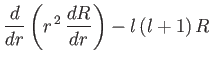
It is easily seen that
 |
(7.15) |
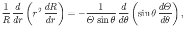
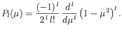
which can only be satisfied provided
where
 , and
, and  is a constant. The solutions to Equation (7.17) that are well behaved for
  in the range
 to
to  are known as the Legendre polynomials, and are denoted the
  ), where
 is a non-negative integer (Jackson 1962). (If
is non-integer then the solutions are singular at
is a non-negative integer (Jackson 1962). (If
is non-integer then the solutions are singular at
 ) In fact,
 |
(7.18) |
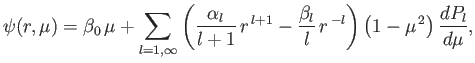
Hence,
 |
 |
(7.19) |
 |
 |
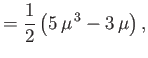
(7.20) |
 |
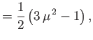 |
(7.21) |
 |
 |
(7.22) |
et cetera. The general solution of Equation (7.16) is a linear combination of  and
and
 factors.
Thus, the general axisymmetric solution of Equation (7.12) is written
factors.
Thus, the general axisymmetric solution of Equation (7.12) is written
![$\displaystyle \phi(r,\theta) = \sum_{l=0,\infty} \left[\alpha_l\,r^{\,l} + \beta_l\,r^{-(l+1)}\right]P_l(\cos\theta),$](img2594.png) |
(7.23) |
where the  and
and  are arbitrary coefficients. It follows from Equations (7.4) that the
corresponding expression for the Stokes stream function is
are arbitrary coefficients. It follows from Equations (7.4) that the
corresponding expression for the Stokes stream function is
 |
(7.24) |
where
.
Next: Uniform Flow
Up: Axisymmetric Incompressible Inviscid Flow
Previous: Axisymmetric Velocity Fields
Richard Fitzpatrick
2016-03-31
![$\displaystyle \frac{d}{d\mu}\left[(1-\mu^{\,2})\,\frac{d{\mit\Theta}}{d\mu}\right]+l\,(l+1)\,{\mit\Theta}$](img2576.png)