


Next: Cylindrical Coordinates
Up: Non-Cartesian Coordinates
Previous: Introduction
Let  ,
,  ,
,  be a set of standard right-handed Cartesian coordinates. Furthermore, let
 ,
,
 ,
,
 be three independent functions of these coordinates which are
such that each unique triplet of
,
,
values is associated with a unique triplet of
be three independent functions of these coordinates which are
such that each unique triplet of
,
,
values is associated with a unique triplet of
 ,
,  ,
,  values. It follows that
,
,
can be used as an alternative set of coordinates to
distinguish different points in space. Because the surfaces of constant
,
, and
are not
generally parallel planes, but rather curved surfaces, this type of coordinate system is termed curvilinear.
values. It follows that
,
,
can be used as an alternative set of coordinates to
distinguish different points in space. Because the surfaces of constant
,
, and
are not
generally parallel planes, but rather curved surfaces, this type of coordinate system is termed curvilinear.
Let
 ,
,
 , and
, and
 . It follows that
 ,
,
 , and
, and
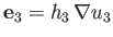 are
a set of unit basis vectors that are normal to surfaces of constant
,
, and
, respectively, at all points
in space. Note, however, that the direction of these basis vectors is generally a function of position. Suppose that
the
are
a set of unit basis vectors that are normal to surfaces of constant
,
, and
, respectively, at all points
in space. Note, however, that the direction of these basis vectors is generally a function of position. Suppose that
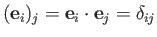
the  , where
  runs from 1 to 3, are mutually orthogonal at all points in space: that is,
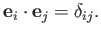 |
(C.1) |
In this case,
,
,
are said to constitute an orthogonal coordinate system.
Suppose, further, that
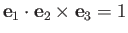 |
(C.2) |
at all points in space, so that
,
,
also constitute a right-handed
coordinate system. It follows that
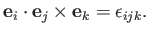 |
(C.3) |
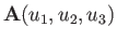
Finally, a general vector  , associated with a particular point in space, can be written
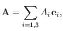 |
(C.4) |
where the
are the local basis vectors of the
,
,
system, and
 is termed the
th component of
in this system.
is termed the
th component of
in this system.
Consider two neighboring points in space whose coordinates in the
,
,
system are
,
,
and  ,
,  ,
,  .
It is easily shown that the vector directed from the first to the second of these points takes the form
.
It is easily shown that the vector directed from the first to the second of these points takes the form
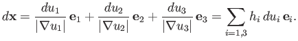 |
(C.5) |
Hence, from (C.1), an element of length (squared) in the
,
,
coordinate system is written
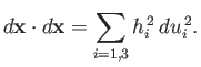 |
(C.6) |
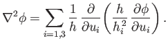
Here, the  , which are generally functions of position, are known as the scale factors of the system.
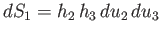
Elements of area that are normal to
, which are generally functions of position, are known as the scale factors of the system.
Elements of area that are normal to  ,
,  , and
, and  , at a given point in space, take the form
 ,
,
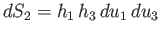 , and
, and
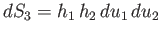 , respectively. Finally, an element of
volume, at a given point in space, is written
, respectively. Finally, an element of
volume, at a given point in space, is written
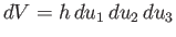 , where
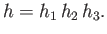 |
(C.7) |
It can be seen that [see Equation (A.176)]
 |
(C.8) |
and
 |
(C.9) |
The latter result follows from Equations (A.175) and (A.176) because
 ,
et cetera. Finally, it is easily demonstrated from Equations (C.1) and (C.3) that
,
et cetera. Finally, it is easily demonstrated from Equations (C.1) and (C.3) that
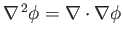
Consider a scalar field
 . It follows from the chain rule, and the relation
 ,
that
,
that
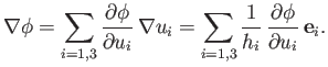 |
(C.12) |
Hence, the components of
 in the
,
,
coordinate system are
in the
,
,
coordinate system are
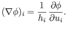 |
(C.13) |
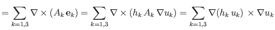
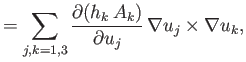
Consider a vector field
 . We can write
where use has been made of Equations (A.174), (C.9), and (C.10). Thus, the
divergence of
in the
,
,
coordinate system takes the form
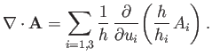 |
(C.15) |
We can write
where use has been made of Equations (A.178), (C.8), and (C.12).
It follows from Equation (C.11) that
 |
(C.17) |
Hence, the components of
 in the
,
,
coordinate system are
in the
,
,
coordinate system are
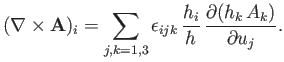 |
(C.18) |
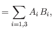
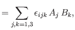
Now,
 [see Equation (A.172)], so Equations (C.12) and (C.15)
yield the following expression for
[see Equation (A.172)], so Equations (C.12) and (C.15)
yield the following expression for
 in the
,
,
coordinate system:
in the
,
,
coordinate system:
 |
(C.19) |
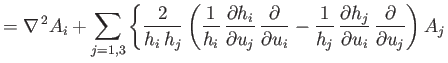
The vector identities (A.171) and (A.179) can be combined to give the
following expression for
 that is valid in a general coordinate system:
Making use of Equations (C.13), (C.15), and (C.18), as well
as the easily demonstrated results
and the tensor identity (B.16), Equation (C.20) reduces (after a great deal of tedious algebra) to the
following expression for the components of
in the
,
,
coordinate system:
![$\displaystyle [({\bf A}\cdot\nabla)\,{\bf B}]_i= \sum_{j=1,3}\left(\frac{A_j}{h...
...ial u_i} + \frac{A_i\,B_j}{h_i\,h_j}\,\frac{\partial h_i}{\partial u_j}\right).$](img7088.png) |
(C.23) |
Note, incidentally, that the commonly quoted result
![$ [({\bf A}\cdot\nabla)\,{\bf B}]_i={\bf A}\cdot\nabla B_i$](img7089.png) is only valid in Cartesian coordinate systems (for which
is only valid in Cartesian coordinate systems (for which
 ).
).
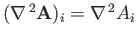
Let us define the gradient
 of a vector field
as the tensor whose components in a Cartesian coordinate
system take the form
of a vector field
as the tensor whose components in a Cartesian coordinate
system take the form
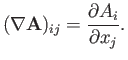 |
(C.24) |
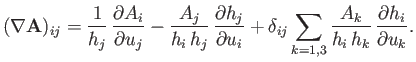
In an orthogonal curvilinear coordinate system, the previous
expression generalizes to
![$\displaystyle (\nabla{\bf A})_{ij} = [({\bf e}_j\cdot\nabla)\,{\bf A}]_i.$](img7093.png) |
(C.25) |
It thus follows from Equation (C.23), and the relation
 , that
 |
(C.26) |
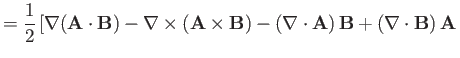
The vector identity (A.177) yields the
following expression for
 that is valid in a general coordinate system:
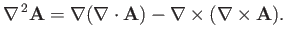 |
(C.27) |
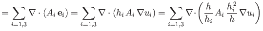
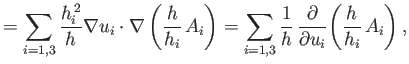
Making use of Equations (C.15), (C.18), and (C.19), as well
as (C.21) and (C.22), and the tensor identity (B.16), the previous equation reduces (after a great deal of
tedious algebra) to the following expression for the components of
in the
,
,
coordinate system:
Note, again, that the commonly quoted result
 is only valid in Cartesian coordinate systems (for which
 ).
).
Next: Cylindrical Coordinates
Up: Non-Cartesian Coordinates
Previous: Introduction
Richard Fitzpatrick
2016-03-31
![$\displaystyle \phantom{=}+\frac{h}{h_i\,h_j^{\,2}}\left[\frac{A_j}{h_i^{\,2}}\,...
... u_j}\,\frac{\partial}{\partial u_j}\!\left( \frac{h_j^{\,2}}{h}\right) \right]$](img7100.png)
![$\displaystyle \phantom{=}+\frac{A_j}{h_i}\,\frac{h}{h_j^{\,3}}\left[\frac{1}{h_...
...ial^{\,2}}{\partial u_i\,\partial u_j}\!\left(\frac{h_j^{\,2}}{h}\right)\right]$](img7101.png)
![$\displaystyle \phantom{=}\left.-\frac{A_i}{h_i\,h_j^{\,2}}\left[\frac{2}{h_i}\l...
...partial u_j}\right)^2-\frac{\partial^2 h_i}{\partial u_j^{\,2}}\right]\right\}.$](img7102.png)