| (5.1) |
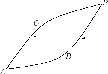
Let ![]() be a fixed point in the
be a fixed point in the ![]() -
-![]() plane, and let
plane, and let ![]() and
and ![]() be two curves, also in the
be two curves, also in the ![]() -
-![]() plane,
that join
plane,
that join ![]() to an arbitrary point
to an arbitrary point ![]() . (See Figure 5.1.) Suppose that fluid is neither created nor destroyed in the region,
. (See Figure 5.1.) Suppose that fluid is neither created nor destroyed in the region, ![]() (say), bounded by
these curves. Because the fluid is incompressible, which essentially means that its density is uniform and constant,
fluid continuity requires that the rate at which the fluid flows into the region
(say), bounded by
these curves. Because the fluid is incompressible, which essentially means that its density is uniform and constant,
fluid continuity requires that the rate at which the fluid flows into the region ![]() , from right to left (in Figure 5.1) across the
curve
, from right to left (in Figure 5.1) across the
curve ![]() , is equal to the rate at which it flows out the of the region, from right to left across the
curve
, is equal to the rate at which it flows out the of the region, from right to left across the
curve ![]() . The rate of fluid flow across a surface is generally termed the flux. Thus, the flux (per unit length parallel to the
. The rate of fluid flow across a surface is generally termed the flux. Thus, the flux (per unit length parallel to the ![]() -axis) from right to left across
-axis) from right to left across ![]() is equal to the flux from right to left across
is equal to the flux from right to left across ![]() . Because
. Because ![]() is arbitrary, it follows that the flux from right to left across any curve
joining points
is arbitrary, it follows that the flux from right to left across any curve
joining points ![]() and
and ![]() is equal to the flux from right to left across
is equal to the flux from right to left across ![]() . In fact, once the base point
. In fact, once the base point ![]() has been chosen, this flux only depends on the position of point
has been chosen, this flux only depends on the position of point ![]() , and the time
, and the time ![]() . In other words, if we denote the flux by
. In other words, if we denote the flux by ![]() then
it is solely a function of the location of
then
it is solely a function of the location of ![]() and the time. Thus, if point
and the time. Thus, if point ![]() lies at the origin, and point
lies at the origin, and point ![]() has Cartesian
coordinates (
has Cartesian
coordinates (![]() ,
, ![]() ), then we can write
), then we can write
| (5.2) |
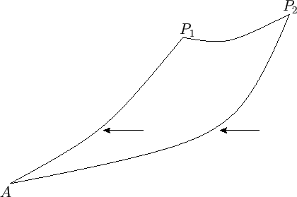
Consider two points, ![]() and
and ![]() , in addition to the fixed point
, in addition to the fixed point ![]() . (See Figure 5.2.) Let
. (See Figure 5.2.) Let ![]() and
and ![]() be the fluxes
from right to left across curves
be the fluxes
from right to left across curves ![]() and
and ![]() . Using similar arguments to those employed previously, the
flux across
. Using similar arguments to those employed previously, the
flux across ![]() is equal to the flux across
is equal to the flux across ![]() plus the flux across
plus the flux across ![]() . Thus, the
flux across
. Thus, the
flux across ![]() , from right to left, is
, from right to left, is
![]() . If
. If ![]() and
and ![]() both lie on the same streamline
then the flux across
both lie on the same streamline
then the flux across ![]() is zero, because the local fluid velocity is directed everywhere parallel to
is zero, because the local fluid velocity is directed everywhere parallel to ![]() . It follows that
. It follows that
![]() . Hence, we conclude that the
stream function is constant along a streamline. The equation of a streamline is thus
. Hence, we conclude that the
stream function is constant along a streamline. The equation of a streamline is thus ![]() , where
, where ![]() is an arbitrary constant.
is an arbitrary constant.
Let
![]() be an infinitesimal arc of a curve that is sufficiently short that it can be regarded as a straight-line.
The fluid velocity in the vicinity of this arc can be resolved into components parallel and perpendicular to the arc.
The component parallel to
be an infinitesimal arc of a curve that is sufficiently short that it can be regarded as a straight-line.
The fluid velocity in the vicinity of this arc can be resolved into components parallel and perpendicular to the arc.
The component parallel to ![]() contributes nothing to the flux across the arc from right to left. The component perpendicular to
contributes nothing to the flux across the arc from right to left. The component perpendicular to
![]() contributes
contributes
![]() to the flux. However, the flux is equal to
to the flux. However, the flux is equal to
![]() . Hence,
. Hence,
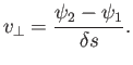 |
(5.3) |
 |
(5.4) |
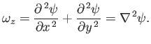
The vorticity in two-dimensional flow takes the form
| (5.8) |
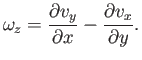 |
(5.9) |
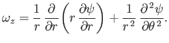
When expressed in terms of cylindrical coordinates (see Section C.3), Equation (5.7) yields
| (5.12) |