Next: Crocco's Theorem
Up: Two-Dimensional Compressible Inviscid Flow
Previous: Shock-Expansion Theory
Thin-Airfoil Theory
The shock-expansion theory of the previous section provides a simple and general method for computing the lift and
drag on a supersonic airfoil, and is applicable as long as the flow is not compressed to subsonic speeds, and the shock
waves remain attached to the airfoil. However, the results of this theory cannot generally be expressed in concise
analytic form. In fact, the theory is mostly used to obtain numerical solutions. However, if the airfoil is thin, and
the angle of attach small, then the shocks and expansion fans attached to the airfoil become weak. In this situation,
shock-expansion theory can be considerably simplified by using approximate expressions for weak shocks and expansion
fans.
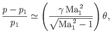
The basic approximate expression [cf. Equation (15.19)]
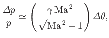 |
(15.46) |
specifies the relative change in pressure across either a weak oblique shock (see Section 15.4) or a weak expansion fan (see Exercise vi) that deflects flow
of Mach number  through an angle
 . Because, in the weak wave approximation, the pressure,
 , never greatly differs from the upstream pressure,
  , and the Mach number,
, never differs appreciably from the
upstream Mach number,
, and the Mach number,
, never differs appreciably from the
upstream Mach number,
 , we can write
 |
(15.47) |
which is correct to first order in  . Here,
is the deflection angle relative to the upstream flow.
. Here,
is the deflection angle relative to the upstream flow.
It is convenient to define a dimensionless quantity known as the pressure coefficient:
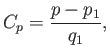 |
(15.48) |
where
 , and
, and  and
and  are the upstream density and flow speed, respectively. Given that the upstream sound speed is
 , and
, and
 , we obtain
 |
(15.49) |
which yields
 |
(15.50) |
This is the fundamental formula of thin-airfoil theory. It states that the pressure coefficient is proportional to the
local deflection of the flow from the upstream direction.
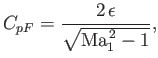
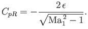
Consider the flat-plate airfoil shown in Figure 15.10. The deflection angle is  on the upper surface of the
airfoil, and
on the upper surface of the
airfoil, and  on the lower surface. (A positive deflection angle corresponds to compression, and a negative deflection
angle to expansion.) Thus, the pressure coefficients on the upper and lower surfaces are
on the lower surface. (A positive deflection angle corresponds to compression, and a negative deflection
angle to expansion.) Thus, the pressure coefficients on the upper and lower surfaces are
 |
(15.51) |
and
 |
(15.52) |
respectively.
It is convenient to define the dimensionless coefficient of lift,
 |
(15.53) |
and the dimensionless coefficient of drag,
 |
(15.54) |
It follows that
Making use of Equations (15.51) and (15.52), as well as the conventional small angle approximations
 and
and
 , we obtain
The focus (see Section 9.3) of the airfoil is at the midchord. Moreover, the ratio
 is
independent of
is
independent of  .
.
Figure:
A diamond-section airfoil.
is the upstream Mach number.  and
and  denote pressures.
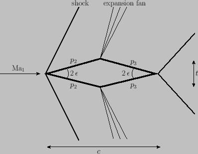 |
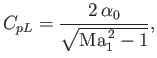
As a second example, consider the diamond-section airfoil pictured in Figure 15.11. This airfoil
has a nose angle
 , and zero angle of attack. The pressure coefficient on the front
face of the airfoil is
, and zero angle of attack. The pressure coefficient on the front
face of the airfoil is
 |
(15.59) |
whereas that on the rear face is
 |
(15.60) |
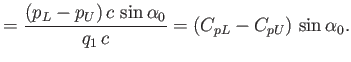
It follows that the pressure difference is
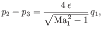 |
(15.61) |
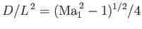
giving a drag
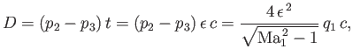 |
(15.62) |
where  and
and  are the thickness and chord-length of the airfoil, respectively. (See Figure 15.11.) Thus,
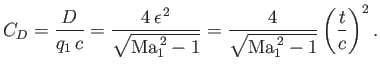 |
(15.63) |
Figure 15.12:
An arbitrary airfoil.
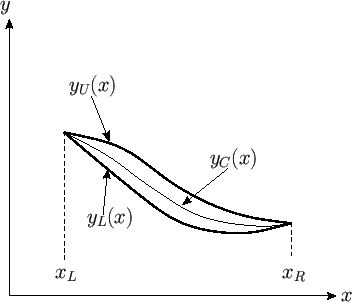 |
Figure 15.12 shows the cross-section of an arbitrary airfoil. The cross-section is assumed to be uniform in the  -direction, with the upstream flow parallel to the
  -axis. The upper surface of the
airfoil corresponds to the curve
-axis. The upper surface of the
airfoil corresponds to the curve  , the lower surface to the curve
  , and the camber line (i.e., the centerline) to the curve
  . Furthermore, the leading and
trailing edges of the airfoil lie at
. Furthermore, the leading and
trailing edges of the airfoil lie at  and
and  , respectively. Hence,
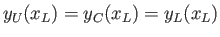 and
and
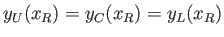 .
By definition,
.
By definition,
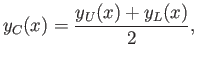 |
(15.64) |
for
 . It is helpful to define the half-width of the airfoil,
 |
(15.65) |
for
. Note that
 . We can also
define the mean angle of attack of the airfoil:
. We can also
define the mean angle of attack of the airfoil:
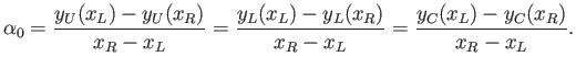 |
(15.66) |
Thus, we can write
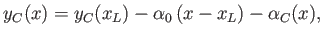 |
(15.67) |
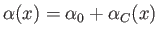
where
 . Here,
 |
(15.68) |
is the local angle of attack of the camber line.
Thus, the camber function,
 , parameterizes the deviations of
  from
across the width of the airfoil.
Equations (15.64), (15.65), and (15.67) yield
from
across the width of the airfoil.
Equations (15.64), (15.65), and (15.67) yield
Hence, the airfoil shape is completely specified by the thickness function,  , the camber function,
, and the
mean angle of attack,
.
, the camber function,
, and the
mean angle of attack,
.
The pressure coefficients on the
upper and lower surfaces of the airfoil are [see Equations (15.50)]
respectively.
It follows from Equations (15.68)-(15.70) that
Now, the lift and drag per unit transverse length acting on the airfoil are given by [cf., Equations (15.53)-(15.56)]
Thus, it follows from Equations (15.71)-(15.74) that
It is helpful to define the chord-average operator:
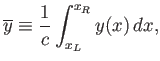 |
(15.79) |
where  is the chord-length. Taking the average of Equation (15.73), making use of Equation (15.66), as well as the
fact that
, we obtain
is the chord-length. Taking the average of Equation (15.73), making use of Equation (15.66), as well as the
fact that
, we obtain
 |
(15.80) |
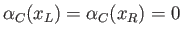
However, the average of Equation (15.68) yields
 |
(15.81) |
which implies that
 .
We can also write
.
We can also write
 |
(15.82) |
Hence, the coefficients of lift and drag,
 and
and
 , are written
respectively.
Thus, in thin-airfoil theory, the lift only depends on the mean angle of attack, whereas the drag splits into three components. Namely, a
drag due to thickness, a drag due to lift, and a drag due to camber.
Next: Crocco's Theorem
Up: Two-Dimensional Compressible Inviscid Flow
Previous: Shock-Expansion Theory
Richard Fitzpatrick
2016-01-22
![$\displaystyle = q_1\int_{x_L}^{x_R} \left[C_{pL}\left(-\frac{dy_L}{dx}\right)+C_{pU}\left(\frac{dy_U}{dy}\right)\right]dx.$](img5843.png)
![$\displaystyle = \frac{2\,q_1}{\sqrt{{\rm Ma}_1^{\,2}-1}}\int_{x_L}^{x_R}\left[\left(\frac{dy_L}{dx}\right)^2+\left(\frac{dy_U}{dx}\right)^2\right]dx$](img5845.png)
![$\displaystyle = \frac{4\,q_1}{\sqrt{{\rm Ma}_1^{\,2}-1}}\int_{x_L}^{x_R}\left[\left(\frac{dh}{dx}\right)^2+\alpha^{\,2}\right]dx.$](img5846.png)
![$\displaystyle = \frac{4}{\sqrt{{\rm Ma}_1^{\,2}-1}}\left[\,\overline{\left(\frac{dh}{dx}\right)^2}+\overline{\alpha^{\,2}}\right]$](img5856.png)
![$\displaystyle =\frac{4}{\sqrt{{\rm Ma}_1^{\,2}-1}}\left[\, \overline{\left(\frac{dh}{dx}\right)^2}+\alpha_0^{\,2}+\overline{\alpha_C^{\,2}}\right],$](img5857.png)