


Next: Laplace Tidal Equations
Up: Terrestrial Ocean Tides
Previous: Total Gravitational Potential
Planetary Response
The interior of the planet is modeled as a uniform, incompressible, elastic, solid possessing the stress-strain relation (Love 1927)
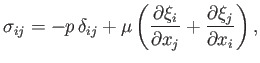 |
(12.60) |
and subject to the incompressibility constraint
Here,
 is the stress tensor,
 the identity tensor,

 the elastic displacement,
 the pressure, and
  the (uniform) rigidity of the material making up the planet (Riley 1974).
The planet's equation of elastic motion in the
co-rotating frame is (Fitzpatrick 2012)
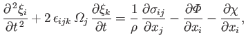 |
(12.62) |
where
 is the totally antisymmetric tensor (Riley 1974), and (Fitzpatrick 2012)
Note that
 is a solid harmonic of degree
  .
The second term on the left-hand side of Equation (12.62) is the Coriolis acceleration (due to planetary rotation), whereas the final
term on the right-hand side is the centrifugal acceleration (likewise, due to planetary rotation). The first two terms on the
right-hand side are the forces per unit mass due to internal stresses and gravity, respectively.
.
The second term on the left-hand side of Equation (12.62) is the Coriolis acceleration (due to planetary rotation), whereas the final
term on the right-hand side is the centrifugal acceleration (likewise, due to planetary rotation). The first two terms on the
right-hand side are the forces per unit mass due to internal stresses and gravity, respectively.
Equations (12.60), (12.61), and (12.62) can be combined to give
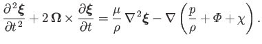 |
(12.66) |
Let us assume that
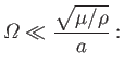 |
(12.67) |
that is, the typical timescale on which the tide generating potential varies (in the co-rotating frame) is much longer than the transit time
of an elastic shear wave through the interior of the planet. In this case, we can neglect the left-hand side of Equation (12.66), and
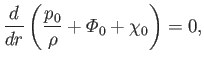
write
which is equivalent to saying that the interior of the planet always remains in an equilibrium state.
Let
![$\displaystyle p(r,\theta,\phi) = p_0(r) + \sum_{n=1,\infty}\left[p_n(r,\theta,\...
...ho\,{\mit\Phi}_n(r,\theta,\phi)\right]-\rho\,\mit\Phi_{\rm ext}(r,\theta,\phi),$](img4385.png) |
(12.69) |
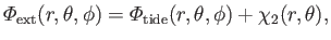
where
 |
(12.70) |
is the sum of the tide generating potential and the fictitious centrifugal potential due to planetary rotation.
Note that
 is a solid harmonic of degree 2.
It follows from Equations (12.50), (12.63), and (12.68) that
is a solid harmonic of degree 2.
It follows from Equations (12.50), (12.63), and (12.68) that
 |
(12.71) |
and
Taking the divergence of the previous equation, and making use of Equations (12.61), we find that
 , which implies
that
, which implies
that
 is a solid harmonic (of degree
  ).
).
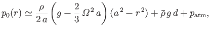
Equation (12.71) can be integrated to give
 |
(12.73) |
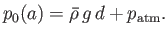
where use has been made of Equations (12.55) and (12.64), as well as
 |
(12.74) |
Here,
 is the atmospheric pressure at sea level.
The previous boundary condition ensures that the mean pressure at the surface of the planet is able to support the mean weight of the ocean, as
well as the weight of the atmosphere.
Incidentally, it is assumed that
is the atmospheric pressure at sea level.
The previous boundary condition ensures that the mean pressure at the surface of the planet is able to support the mean weight of the ocean, as
well as the weight of the atmosphere.
Incidentally, it is assumed that
 , and we have neglected terms of order
 with respect to terms of order
 .
.
The elastic displacement in the interior of the planet satisfies Equations (12.61) and (12.72). It is helpful to define the radial
component of the displacement
 |
(12.75) |
as well as the stress acting (outward) across a constant  surface,
![$\displaystyle X_i= -\frac{x_j\,\sigma_{ij}}{r} = p\,\frac{x_i}{r} - \frac{\mu}{...
...ial \xi_i}{\partial r}-\xi_i + \frac{\partial (r\,\xi_r)}{\partial x_i}\right],$](img4400.png) |
(12.76) |
where use has been made of Equation (12.60).
The radial displacement at  is equivalent to the displacement of the planet's surface.
Hence, according to Equation (12.45),
is equivalent to the displacement of the planet's surface.
Hence, according to Equation (12.45),
 |
(12.77) |
The stress at any point on the surface
must be entirely radial (because a fluid ocean cannot withstand a tangential stress), and such as to balance the weight of the column of rock and ocean directly above the point in question. In other words,
![$\displaystyle X_i(a,\theta,\phi) = g\left[\rho\,\zeta_b + \skew{3}\bar{\rho}\,(d+\zeta)\right]\left(\frac{x_i}{r}\right)_{r=a}.$](img4402.png) |
(12.78) |
It follows from Equation (12.57), (12.69), (12.70), (12.74), (12.76), and (12.78)
that
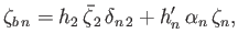
where
 |
(12.79) |
is a surface harmonic of degree
. Here,
 , which has the dimensions of length, parameterizes the perturbation due to tidal and
rotational effects at the planet's surface. Moreover,
, which has the dimensions of length, parameterizes the perturbation due to tidal and
rotational effects at the planet's surface. Moreover,
 is a Kronecker delta symbol (Riley 1974).
Hence, we need to solve Equations (12.61) and (12.72), subject to the boundary conditions (12.77) and (12.79).
is a Kronecker delta symbol (Riley 1974).
Hence, we need to solve Equations (12.61) and (12.72), subject to the boundary conditions (12.77) and (12.79).
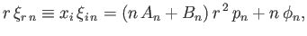
Let us try a solution to Equations (12.61) and (12.72) of the form
 |
(12.80) |
where (Love 1927)
 |
(12.81) |
Here,  and
and  are spatial constants, and
 is an arbitrary solid harmonic of degree
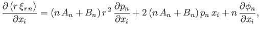
. It follows that
is an arbitrary solid harmonic of degree
. It follows that
 |
(12.82) |
where use has been made of Equation (12.40). Moreover,
 |
(12.83) |
and
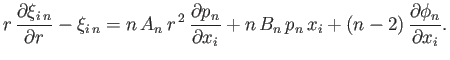 |
(12.84) |
Thus, the boundary conditions (12.77) and (12.79)
become
![$\displaystyle \left[(2\,A_n+B_n)\,r^{\,2}\,p_n + n\,\phi_n\right]_{r=a} = a\,\zeta_{b\,n},$](img4415.png) |
(12.85) |
and
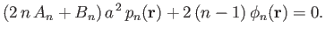
respectively. Suppose that
is such that
 |
(12.86) |
In this case, the boundary conditions (12.86) and (12.87) reduce to
![$\displaystyle \left[\frac{-4\,A_n+(n-2)\,B_n}{2\,(n-1)}\right]a\left.p_n\right\vert _{r=a} = \zeta_{b\,n},$](img4418.png) |
(12.87) |
and
respectively.
The expression for
 given in Equation (12.82) satisfies Equations (12.61) and (12.72) provided that
respectively, where use has been made of Equations (12.40)-(12.42). It follows that
Hence, the boundary conditions (12.89) and (12.90) yield
 |
(12.92) |
where
Here, the  parameterize the self-gravity of the ocean.
Let
parameterize the self-gravity of the ocean.
Let
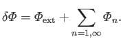 |
(12.96) |
This quantity can be recognized as the total perturbing potential at the planet's surface due to the combination of tidal, rotational, and ocean self-gravity, effects.
It follows from Equation (12.57), (12.80), and (12.95) that
![$\displaystyle - \left(\frac{\delta {\mit\Phi}}{g}\right)_{r=a} =\sum_{n=1,\inft...
..._2)\,\skew{5}\bar{\zeta}_2\,\delta_{n\,2} + (1+k_n')\,\alpha_n\,\zeta_n\right],$](img4436.png) |
(12.97) |
where
Here, the dimensionless quantities  ,
,  ,
,  , and
, and  are known as Love numbers (Love 1911).
Next: Laplace Tidal Equations
Up: Terrestrial Ocean Tides
Previous: Total Gravitational Potential
Richard Fitzpatrick
2016-01-22
![\begin{multline}
\left(\sum_{n=1,\infty}p_n\,\frac{x_i}{r} - \frac{\mu}{r}\left[...
...ar{\rho}}{\rho}\,\zeta_n\right]\left(\frac{x_i}{r}\right)_{r=a} ,
\end{multline}](img4403.png)
![\begin{multline}
\left(1-[2\,n\,A_n+(2+n)\,B_n]\,\mu\right)\left(p_n\,x_i\right)...
...ight)
\frac{\skew{3}\bar{\rho}}{\rho}\,\zeta_n\right](x_i)_{r=a},
\end{multline}](img4416.png)
![\begin{multline}
\left(1-[2\,n\,A_n+(2+n)\,B_n]\,\mu\right)\left.p_n\right\vert ...
...}{2\,n+1}\right)
\frac{\skew{3}\bar{\rho}}{\rho}\,\zeta_n\right],
\end{multline}](img4419.png)
![$\displaystyle = \left.\left(\frac{2\,n+1}{2\,n-2}\right)\right/\left[1+\frac{(2\,n+1)\,(2\,n^{\,2}+4\,n+3)}{(6+n^{\,2})}\,\frac{\mu}{\rho\,g\,a}\right],$](img4431.png)
![$\displaystyle = -\left.\left(\frac{2\,n+1}{3}\right)\right/\left[1+\frac{(2\,n+1)\,(2\,n^{\,2}+4\,n+3)}{(6+n^{\,2})}\,\frac{\mu}{\rho\,g\,a}\right].$](img4433.png)
![$\displaystyle = \left.\left(\frac{3}{2\,n-2}\right)\right/\left[1+\frac{(2\,n+1)\,(2\,n^{\,2}+4\,n+3)}{(6+n^{\,2})}\,\frac{\mu}{\rho\,g\,a}\right],$](img4438.png)
![$\displaystyle = -\left[1+\frac{(2\,n+1)\,(2\,n^{\,2}+4\,n+3)}{(6+n^{\,2})}\,\frac{\mu}{\rho\,g\,a}\right]^{\,-1}.$](img4440.png)