


Next: Flow Past a Spherical
Up: Axisymmetric Incompressible Inviscid Flow
Previous: Point Sources
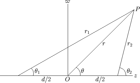
Consider the flow pattern generated by point source of strength  located on the symmetry axis at
  , and
a point source of strength
, and
a point source of strength  (i.e., a point sink) located on the symmetry axis at
  .
It follows, by analogy with the analysis of the previous section, that the stream function and velocity potential at a general
point,
.
It follows, by analogy with the analysis of the previous section, that the stream function and velocity potential at a general
point,  , lying in the meridian plane, are
 |
(7.36) |
and
 |
(7.37) |
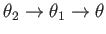
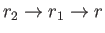
respectively. Here,  ,
,  ,
,  , and
, and  are defined in Figure 7.2.
Figure 7.2:
A dipole source.
 |
In the limit that the product  remains constant, while
 , we obtain a so-called dipole point source.
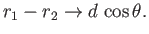
According to the sine rule of trigonometry,
, we obtain a so-called dipole point source.
According to the sine rule of trigonometry,
 |
(7.38) |
However,
![$ \sin(\theta_2-\theta_1)= 2\,\sin[(\theta_2-\theta_1)/2]\,\cos[(\theta_2-\theta_1)/2]$](img2623.png) , so
we obtain
, so
we obtain
![$\displaystyle r_1-r_2 = \frac{d\,(\sin\theta_2-\sin\theta_1)}{2\,\sin[(\theta_2-\theta_1)/2]\,\cos[(\theta_2-\theta_1)/2]}.$](img2624.png) |
(7.39) |
In fact,
![$ \sin\theta_2-\sin\theta_1 = 2\,\cos[(\theta_2+\theta_1)/2]\,\sin[(\theta_2-\theta_1)/2]$](img2625.png) ,
which leads to
,
which leads to
![$\displaystyle r_1 - r_2= \frac{d\,\cos[(\theta_2+\theta_1)/2]}{\cos[(\theta_2-\theta_1)/2]}.$](img2626.png) |
(7.40) |
Thus, in the limit
 and
and
 ,
we get
,
we get
 |
(7.41) |
Hence, according to Equation (7.37),
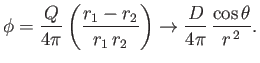 |
(7.42) |
Equation (7.36) implies that
![$\displaystyle \psi = \frac{Q}{4\pi}\left(\frac{z-d/2}{r_2}-\frac{z+d/2}{r_1}\ri...
...frac{1}{r_1}\right)-\frac{d}{2}\left(\frac{1}{r_2}+\frac{1}{r_1}\right)\right].$](img2631.png) |
(7.43) |
Thus, in the limit
and
,
we obtain
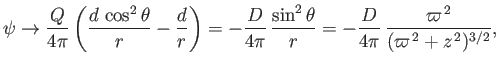 |
(7.44) |
where use has been made of Equation (7.41), as well as the fact that
 .
Figure 7.3 shows the stream function of a dipole point source located at the origin.
.
Figure 7.3 shows the stream function of a dipole point source located at the origin.
Figure 7.3:
Contours of the stream function of a dipole source located at the origin.
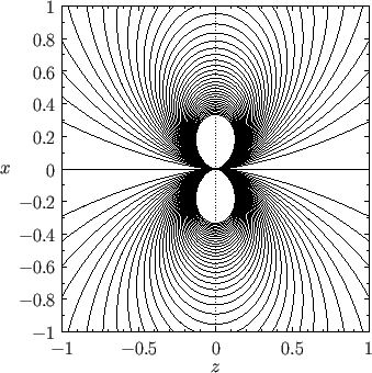 |
Incidentally, Equations (7.26), (7.28), (7.33), (7.35), (7.42), and (7.44) imply that the terms in the
expansions (7.23) and (7.24) involving the constants  ,
,  , and
, and  correspond to
a point source at the origin, uniform flow parallel to the
correspond to
a point source at the origin, uniform flow parallel to the  -axis, and a dipole point source at the origin, respectively.
Of course, the term involving
-axis, and a dipole point source at the origin, respectively.
Of course, the term involving  is constant, and, therefore, gives rise to no flow.
Next: Flow Past a Spherical
Up: Axisymmetric Incompressible Inviscid Flow
Previous: Point Sources
Richard Fitzpatrick
2016-01-22