


Next: Example 2-d electrostatic calculation
Up: Poisson's equation
Previous: An example 2-d Poisson
Let us now use the techniques discussed above to solve Poisson's
equation in two dimensions. Suppose that the source term is
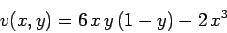 |
(181) |
for
 and
and
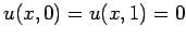
 . The boundary conditions
at
. The boundary conditions
at  are
are  ,
,  , and
, and  [see Eq. (147)], whereas
the boundary conditions at
[see Eq. (147)], whereas
the boundary conditions at  are
are  ,
,  ,
and
,
and
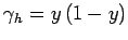 [see Eq. (148)]. The simple Dirichlet boundary
conditions
[see Eq. (148)]. The simple Dirichlet boundary
conditions
 are applied at
  and
and  . Of course,
this problem can be solved analytically to give
. Of course,
this problem can be solved analytically to give
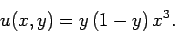 |
(182) |
Figures 63 and 64 show comparisons between the analytic and finite difference
solutions for  . It can be seen that the finite difference solution mirrors
the analytic solution almost exactly.
. It can be seen that the finite difference solution mirrors
the analytic solution almost exactly.
Figure 63:
Solution of Poisson's equation in two dimensions with simple
Dirichlet boundary conditions in the  -direction. The solution is plotted versus
  at
at
 .
The dotted curve (obscured)
shows the analytic solution, whereas the open triangles show the finite difference
solution for .
.
The dotted curve (obscured)
shows the analytic solution, whereas the open triangles show the finite difference
solution for .
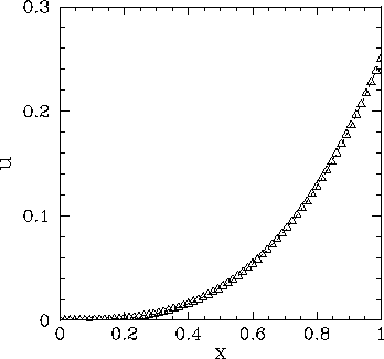 |
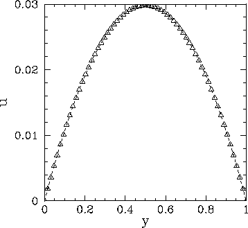
Figure 64:
Solution of Poisson's equation in two dimensions with simple
Dirichlet boundary conditions in the -direction. The solution is plotted versus at
 .
The dotted curve (obscured)
shows the analytic solution, whereas the open triangles show the finite difference
solution for .
.
The dotted curve (obscured)
shows the analytic solution, whereas the open triangles show the finite difference
solution for .
 |
As a second example, suppose that the source term is
 |
(183) |
for
and
. The boundary conditions
at are , , and
 [see Eq. (147)], whereas
the boundary conditions at are , ,
and
[see Eq. (147)], whereas
the boundary conditions at are , ,
and  [see Eq. (148)]. The simple Neumann boundary
conditions
[see Eq. (148)]. The simple Neumann boundary
conditions
 are applied at and . Of course,
this problem can be solved analytically to give
are applied at and . Of course,
this problem can be solved analytically to give
 |
(184) |
Figures 65 and 66 show comparisons between the analytic and finite difference
solutions for . It can be seen that the finite difference solution mirrors
the analytic solution almost exactly.
Figure 65:
Solution of Poisson's equation in two dimensions with simple
Neumann boundary conditions in the -direction. The solution is plotted versus at
.
The dotted curve (obscured)
shows the analytic solution, whereas the open triangles show the finite difference
solution for .
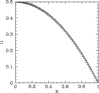 |
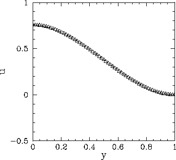
Figure 66:
Solution of Poisson's equation in two dimensions with simple
Neumann boundary conditions in the -direction. The solution is plotted versus at
.
The dotted curve (obscured)
shows the analytic solution, whereas the open triangles show the finite difference
solution for .
 |
Next: Example 2-d electrostatic calculation
Up: Poisson's equation
Previous: An example 2-d Poisson
Richard Fitzpatrick
2006-03-29