 |
We can represent period-1 motion schematically as ![]() , where
, where ![]() represents a pattern
of motion which is repeated every period of the external drive. Likewise, we can represent
period-2 motion as
represents a pattern
of motion which is repeated every period of the external drive. Likewise, we can represent
period-2 motion as ![]() , where
, where ![]() and
and ![]() represent distinguishable patterns of motion
which are repeated every alternate period of the external drive. A period-doubling
bifurcation is represented:
represent distinguishable patterns of motion
which are repeated every alternate period of the external drive. A period-doubling
bifurcation is represented:
![]() . Clearly, all that happens
in such a bifurcation is that the pendulum suddenly decides to do something slightly different in
alternate periods of the external drive.
. Clearly, all that happens
in such a bifurcation is that the pendulum suddenly decides to do something slightly different in
alternate periods of the external drive.
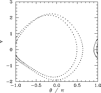 |
Figure 40 shows the time-asymptotic phase-space orbit of the pendulum calculated for a
value of ![]() somewhat higher than that required to trigger the above mentioned period-doubling bifurcation. It can
be seen that the orbit is left-favouring (i.e., it spends the majority of its time on
the left-hand side of the plot), and takes the form of a closed curve consisting of
two interlocked loops in phase-space.
Recall that for period-1 orbits there was only a single closed loop in phase-space.
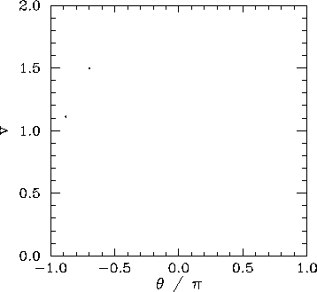
Figure 41 shows the Poincaré section of the orbit shown in Fig. 40.
The fact that the section consists
of two points confirms that the orbit does indeed correspond to period-2 motion.
somewhat higher than that required to trigger the above mentioned period-doubling bifurcation. It can
be seen that the orbit is left-favouring (i.e., it spends the majority of its time on
the left-hand side of the plot), and takes the form of a closed curve consisting of
two interlocked loops in phase-space.
Recall that for period-1 orbits there was only a single closed loop in phase-space.
Figure 41 shows the Poincaré section of the orbit shown in Fig. 40.
The fact that the section consists
of two points confirms that the orbit does indeed correspond to period-2 motion.
 |
A period-doubling bifurcation is an example of temporal symmetry breaking. The equations of
motion of the pendulum are invariant under the transformation
![]() , where
, where
![]() is the period of the external drive. In the low amplitude (i.e., linear) limit
the time-asymptotic motion of the pendulum always respects this symmetry. However, as we have just seen, in the
non-linear regime it is possible to obtain solutions which spontaneously break this symmetry.
Obviously, motion which repeats itself every two periods of the external drive is not
as temporally symmetric as motion which repeats every period of the drive.
is the period of the external drive. In the low amplitude (i.e., linear) limit
the time-asymptotic motion of the pendulum always respects this symmetry. However, as we have just seen, in the
non-linear regime it is possible to obtain solutions which spontaneously break this symmetry.
Obviously, motion which repeats itself every two periods of the external drive is not
as temporally symmetric as motion which repeats every period of the drive.
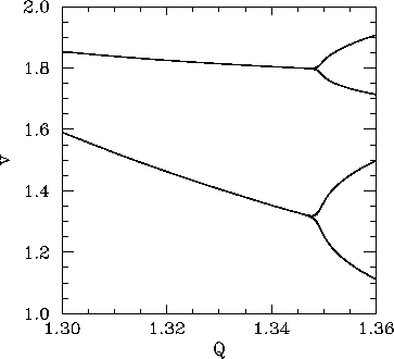 |
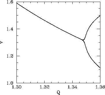
Figure 42 is essentially a continuation of Fig 34. Data is shown for two
sets of initial conditions which lead to motions converging on left-favouring (lower branch) and
right-favouring (upper branch) periodic attractors. We have already seen that the left-favouring
periodic attractor undergoes a period-doubling bifurcation at ![]() . It is clear from Fig. 42
that the right-favouring attractor undergoes a similar bifurcation at almost exactly the
same
. It is clear from Fig. 42
that the right-favouring attractor undergoes a similar bifurcation at almost exactly the
same ![]() -value. This is hardly surprising since, as has already
been mentioned, for fixed physics parameters (i.e.,
-value. This is hardly surprising since, as has already
been mentioned, for fixed physics parameters (i.e., ![]() ,
, ![]() ,
, ![]() ), the
left- and right-favouring attractors are mirror-images of one another.
), the
left- and right-favouring attractors are mirror-images of one another.