Adaptive integration methods

Consider the following system of o.d.e.s:

$$\frac{dx}{dt} = v,$$ (33)

$$\frac{dv}{dt} = \frac{v}{t} - 4\,k\,t^2\,x,$$ (34)

subject to the boundary conditions $x = \sqrt{k}\,\nu^2$ and $v = 2\,\sqrt{k}\,\nu$ at $x=\nu$, where $0<\nu\ll 1$. This system can be solved analytically to give

$$x = \sin(\sqrt{k}\,t^2).$$ (35)

One peculiarity of the above solution is that its variation scale-length decreases rapidly as $t$ increases.

Figure 7: Global integration error associated with a fixed step-length ($h=0.01$), fourth-order Runge-Kutta method, plotted against the independent variable, $t$, for a system of o.d.e.s in which the variation scale-length decreases rapidly with increasing $t$. Double precision calculation.

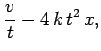
Let us compare the above solution with that obtained numerically using a fourth-order Runge-Kutta method. Figure 7 shows the integration error associated with such a method (calculated by integrating the above system, with $k=10$, from $t=10^{-3}$ to $t=t$, and then taking the difference between the numerical and analytic solutions) with a fixed step-length of $h=0.01$, plotted against the independent variable, $t$. It can be seen that, although the error starts off small, it rises rapidly as the variation scale-length of the solution decreases (i.e., as $t$ increases), and quickly becomes unacceptably large. Of course, we could reduce the error by simply reducing the step-length, $h$. However, this is a very inefficient solution. The step-length only needs to be reduced at large $t$. There is no need to reduce it, at all, at small $t$. Clearly, the ideal solution to this problem would be an integration method in which the step-length is varied so as to maintain a relatively constant truncation error per step. Such an adaptive integration method would take large steps when variation scale-length of the solution was large, and vice versa.

Let us investigate how we could convert our fixed step-length, fourth-order Runge-Kutta method into a corresponding adaptive method. First of all, we need an estimate of the truncation error at each step. Suppose that the current step-length is $h$. We can estimate the truncation error, $\epsilon$, associated with the current step by taking the difference between the solutions obtained by stepping by $h/2$ twice and by $h$ once (starting from the same point, in both cases). Let $\epsilon _0$ be the desired truncation error per step. How do we adjust $h$ so as to ensure that the truncation error associated with the next step is closer to this value? Observe, from Eq. (29), that the truncation error per step in a fourth-order scheme scales like $h^5$. It follows, therefore, that our step-length adjustment formula should take the form¹⁶

$$h_{\rm new} = h_{\rm old}\left\vert\frac{\epsilon_0}{\epsilon}\right\vert^{1/5}.$$ (36)

According to this formula, the step-length should be increased if the truncation error per step is too small, and vice versa, in such a manner that the error per step remains relatively constant at $\epsilon _0$.

There are a number of caveats to the above discussion. In a system of $n$ coupled o.d.e.s, the overall truncation error per step, $\epsilon$, should, of course, be some appropriately weighted average of the errors associated with each equation. There is also a question of whether $\epsilon$ should be an absolute error or a relative error. The relative error associated with the $i$th equation is simply the absolute error divided by $\vert y_i\vert$, where $y_i$ is the current value of the $i$th dependent variable. An absolute error estimate is appropriate to a system of equations in which the amplitudes of the various dependent variables remain bounded. A relative error estimate is appropriate to a system in which the amplitudes of the dependent variables blow-up at some point, but the variables always remain the same sign. Finally, a mixed error estimate--usually the minimum of the absolute and relative errors--is appropriate to a system in which the amplitudes of the dependent variables blow-up at some point, but the signs of the variables oscillate. It is usually a good idea to place some limits on the allowed variation of the step-length from step to step: e.g., by preventing the step-length from increasing or decreasing by more than some factor $S>1$ per step. This prevents $h$ from oscillating unduly about its optimum value. Obviously, if $h$ becomes absurdly small then the integration method has failed, and should abort with an appropriate error message. Finally, a limit should be placed on how large $h$ can become--unfortunately, adaptive methods have a tendency to become a little over optimistic when integration is easy.

Figure 8: Global integration errors associated with a fixed step-length ($h=0.01$), fourth-order Runge-Kutta method (solid curve) and a corresponding adaptive method ( $\epsilon _0=10^{-8}$)(dotted curve), plotted against the independent variable, $t$, for a system of o.d.e.s in which the variation scale-length decreases rapidly with increasing $t$. Double precision calculation.

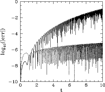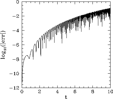
Figure 8 shows the integration errors associated with a fixed step-length, fourth-order Runge-Kutta method and a corresponding adaptive method--constructed along the lines discussed above--as functions of the independent variable, $t$. The errors are calculated by integrating the current system, with $k=10$, from $t=10^{-3}$ to $t=t$, and then taking the difference between the numerical and analytic solutions. The fixed step-length associated with the former method is $h=0.01$. The desired truncation error per step associated with the latter is $\epsilon _0=10^{-8}$. It can be seen that the performance of the adaptive method is far superior to that of the fixed step-length method, since the former method maintains a relatively constant integration error as the variation scale-length of the solution decreases (i.e., as $t$ increases). Figure 9 illustrates how this is achieved. This figure shows the step-length, $h$, associated with the adaptive method as a function of $t$. It can be seen that the adaptive method maintains a relatively constant truncation error per step by decreasing $h$ as $t$ increases.

Figure 9: The step-length, $h$, associated with the adaptive integration method shown in the previous figure, plotted as a function of the independent variable, $t$. Double precision calculation.