An example calculation

Consider the following system of o.d.e.s:

$$\frac{dx}{dt} = v,$$ (30)

$$\frac{dv}{dt} = -k\,x,$$ (31)

subject to the initial conditions $x(0)=0$ and $v(0) = \sqrt{k}$ at $t=0$. In fact, this system can be solved analytically to give

$$x = \sin(\sqrt{k}\,t).$$ (32)

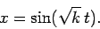
Let us compare the above solution with that obtained numerically using either Euler's method or a fourth-order Runge-Kutta method. Figure 5 shows the integration errors associated with these two methods (calculated by integrating the above system, with $k=1$, from $t=0$ to $t=10$, and then taking the difference between the numerical and analytic solutions) plotted against the step-length, $h$, in a log-log graph. All calculations are performed to single precision: i.e., by using float, rather than double, variables. It can be seen that at large values of $h$, the error associated with Euler's method becomes much greater than unity (i.e., the magnitude of the numerical solution greatly exceeds that of the analytic solution), indicating the presence of a numerical instability. There are no similar signs of instability associated with the Runge-Kutta method. At intermediate $h$, the error associated with Euler's method decreases smoothly like $h^{-1}$: in this regime, the dominant error is truncation error, which is expected to scale like $h^{-1}$ for a first-order method. The error associated with the Runge-Kutta method similarly scales like $h^{-4}$--as expected for a fourth-order scheme--in the truncation error dominated regime. Note that, as $h$ is decreased, the error associated with both methods eventually starts to rise in a jagged curve that scales roughly like $h^1$. This is a manifestation of round-off error. The minimum error associated with both methods corresponds to the boundary between the truncation error and round-off error dominated regimes. Thus, for Euler's method the minimum error is about $10^{-3}$ at $h\sim 10^{-3}$, whereas for the Runge-Kutta method the minimum error is about $10^{-5}$ at $h\sim 10^{-1}$. Clearly, the performance of the Runge-Kutta method is vastly superior to that of Euler's method, since the former method is capable of attaining much greater accuracy than the latter using a far smaller number of steps (i.e., a far larger $h$).

Figure 5: Global integration errors associated with Euler's method (solid curve) and a fourth-order Runge-Kutta method (dotted curve) plotted against the step-length $h$. Single precision calculation.

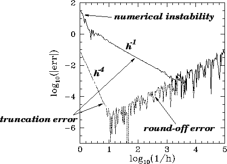Figure 6 displays similar data to that shown in Fig. 5, except that now all of the calculations are performed to double precision. The figure exhibits the same broad features as those apparent in Fig. 5. The major difference is that the round-off error has been reduced by about nine orders of magnitude, allowing the Runge-Kutta method to attain a minimum error of about $10^{-12}$ (see Tab. 1)--a remarkably performance!

Figure 6: Global integration errors associated with Euler's method (solid curve) and a fourth-order Runge-Kutta method (dotted curve) plotted against the step-length $h$. Double precision calculation.

Figures 5 and 6 illustrate why scientists rarely use Euler's method, or single precision numerics, to integrate systems of o.d.e.s.