Euler's method

Consider the general first-order o.d.e.,

$$y' = f(x,y),$$ (5)

where $'$ denotes $d/dx$, subject to the general initial-value boundary condition

$$y(x_0) = y_0.$$ (6)

Clearly, if we can find a method for numerically solving this problem, then we should have little difficulty generalizing it to deal with a system of $n$ simultaneous first-order o.d.e.s.

It is important to appreciate that the numerical solution to a differential equation is only an approximation to the actual solution. The actual solution, $y(x)$, to Eq. (5) is (presumably) a continuous function of a continuous variable, $x$. However, when we solve this equation numerically, the best that we can do is to evaluate approximations to the function $y(x)$ at a series of discrete grid-points, the $x_n$ (say), where $n=0,1,2,\cdots$ and $x_0<x_1<x_2 \cdots$. For the moment, we shall restrict our discussion to equally spaced grid-points, where

$$x_n = x_0 + n\,h.$$ (7)

Here, the quantity $h$ is referred to as the step-length. Let $y_n$ be our approximation to $y(x)$ at the grid-point $x_n$. A numerical integration scheme is essentially a method which somehow employs the information contained in the original o.d.e., Eq. (5), to construct a series of rules interrelating the various $y_n$.

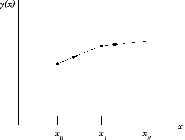
The simplest possible integration scheme was invented by the celebrated 18th century Swiss mathematician Leonhard Euler, and is, therefore, called Euler's method. Incidentally, it is interesting to note that virtually all of the standard methods used in numerical analysis were invented before the advent of electronic computers. In olden days, people actually performed numerical calculations by hand--and a very long and tedious process it must have been! Suppose that we have evaluated an approximation, $y_n$, to the solution, $y(x)$, of Eq. (5) at the grid-point $x_n$. The approximate gradient of $y(x)$ at this point is, therefore, given by

$$y_n' = f(x_n,y_n).$$ (8)

Let us approximate the curve $y(x)$ as a straight-line between the neighbouring grid-points $x_n$ and $x_{n+1}$. It follows that

$$y_{n+1} = y_n + y_n'\,h,$$ (9)

or

$$y_{n+1} = y_n +f(x_n,y_n)\,h.$$ (10)

The above formula is the essence of Euler's method. It enables us to calculate all of the $y_n$, given the initial value, $y_0$, at the first grid-point, $x_0$. Euler's method is illustrated in Fig. 4.

Figure 4: Illustration of Euler's method.