Next: Euler's method
Up: Integration of ODEs
Previous: Integration of ODEs
In this section, we shall discuss the standard numerical techniques
used to integrate systems of ordinary differential equations (ODEs). We shall then employ these
techniques to simulate the trajectories of various different types
of baseball pitch.
By definition, an ordinary differential equation, or o.d.e., is a differential
equation in which all dependent variables are functions of a single independent variable.
Furthermore, an  th-order o.d.e. is such that, when it is reduced to its simplest
form, the highest order derivative it contains is th-order.
th-order o.d.e. is such that, when it is reduced to its simplest
form, the highest order derivative it contains is th-order.
According
to Newton's laws of motion, the motion of any collection of rigid objects can
be reduced to a set of second-order o.d.e.s. in which time,  , is the common independent
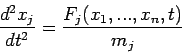
variable. For instance, the equations of motion of a set of interacting point
objects moving in 1-dimension might take the form:
, is the common independent
variable. For instance, the equations of motion of a set of interacting point
objects moving in 1-dimension might take the form:
 |
(2) |
for  to , where
  is the position of the
  th object,
  is
its mass, etc. Note that a set of second-order o.d.e.s can
always be rewritten as a set of
is
its mass, etc. Note that a set of second-order o.d.e.s can
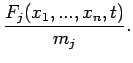
always be rewritten as a set of  first-order o.d.e.s. Thus, the above
equations of motion can be rewritten:
first-order o.d.e.s. Thus, the above
equations of motion can be rewritten:
for to . We conclude that a general knowledge of how to numerically solve a set of
coupled first-order o.d.e.s would enable us to investigate the behaviour of
a wide variety of interesting dynamical systems.
Next: Euler's method
Up: Integration of ODEs
Previous: Integration of ODEs
Richard Fitzpatrick
2006-03-29