Let us extend the analysis of the previous section to consider a general electromagnetic wave
propagating through a uniform plasma with an equilibrium magnetic field of strength,
 . The plasma is assumed to consist of two species: electrons of mass
  and electric
charge
and electric
charge  , and ions of mass
  and electric charge
  . The plasma is also assumed
to be electrically neutral, so that the equilibrium number density of the ions is the same as that of the electrons; namely,
. The plasma is also assumed
to be electrically neutral, so that the equilibrium number density of the ions is the same as that of the electrons; namely,
 (Stix 1962). The equations of motion of a constituent ion of the plasma are written
where
(Stix 1962). The equations of motion of a constituent ion of the plasma are written
where  ,
,  , and
, and  are the wave-induced displacements of the ion along the
three Cartesian axes. (Here, we are including ion motion in our analysis because such
motion is important in certain frequency ranges.)
As before, the former terms on the right-hand sides of the previous equations
represent the forces exerted on the ion by the wave electric field,
are the wave-induced displacements of the ion along the
three Cartesian axes. (Here, we are including ion motion in our analysis because such
motion is important in certain frequency ranges.)
As before, the former terms on the right-hand sides of the previous equations
represent the forces exerted on the ion by the wave electric field,  ,
whereas the latter terms represent the forces exerted by the equilibrium magnetic field when the ion moves (Fitzpatrick 2008). (As before, we can neglect any forces due to the wave magnetic field,
as long as the particle motion remains non-relativistic.)
The equations of motion of a constituent electron take the form
The Cartesian components of the electric dipole moment per unit volume are
Finally, the electric displacement is written
,
whereas the latter terms represent the forces exerted by the equilibrium magnetic field when the ion moves (Fitzpatrick 2008). (As before, we can neglect any forces due to the wave magnetic field,
as long as the particle motion remains non-relativistic.)
The equations of motion of a constituent electron take the form
The Cartesian components of the electric dipole moment per unit volume are
Finally, the electric displacement is written
 |
(9.101) |
Consider a right-hand circularly polarized (with respect to the direction of the equilibrium magnetic field) wave whose electric field takes the form
Let us write
 |
 |
(9.105) |
 |
 |
(9.106) |
 |
 |
(9.107) |
 |
 |
(9.108) |
 |
 |
(9.109) |
 |
|
(9.110) |
 |
 |
(9.111) |
 |
 |
(9.112) |
 |
 |
(9.113) |
 is termed the ion cyclotron frequency, and is the
frequency at which ions gyrate in the plane perpendicular to the equilibrium magnetic field (Stix 1962).
Moreover,
is termed the ion cyclotron frequency, and is the
frequency at which ions gyrate in the plane perpendicular to the equilibrium magnetic field (Stix 1962).
Moreover,
 is the electron cyclotron frequency, and is the
frequency at which electrons gyrate in the plane perpendicular to the equilibrium magnetic field (ibid).
Finally,
is the electron cyclotron frequency, and is the
frequency at which electrons gyrate in the plane perpendicular to the equilibrium magnetic field (ibid).
Finally,
 and
and
 are termed the ion plasma frequency,
and the electron plasma frequency, respectively (ibid). Of course,
are termed the ion plasma frequency,
and the electron plasma frequency, respectively (ibid). Of course,
 and
and
 , because
 .
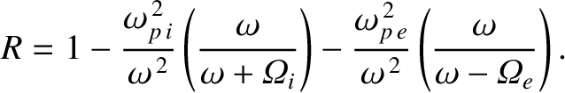
Finally, it follows from Equations (9.101)–(9.104), (9.113), and (9.116), that the electric
displacement of a right-hand circularly polarized wave propagating through a magnetized
plasma has the components
where
.
Finally, it follows from Equations (9.101)–(9.104), (9.113), and (9.116), that the electric
displacement of a right-hand circularly polarized wave propagating through a magnetized
plasma has the components
where
 |
(9.124) |
Consider a left-hand circularly polarized (with respect to the direction of the equilibrium magnetic field) wave whose electric field takes the form
By repeating the previously described analysis (with appropriate modifications), we deduce that
where
 |
(9.131) |
Finally, consider a wave whose electric field is polarized parallel to the equilibrium magnetic field,
so that
Again, repeating the previous analysis (with suitable modifications), we obtain
where
 |
(9.138) |
Now, the equations that govern electromagnetic wave propagation through a
dielectric media are (see Appendix C)
 |
 |
(9.139) |
 |
 |
(9.140) |
 |
 |
(9.141) |
 |
 |
(9.142) |
 |
 |
(9.143) |
 |
 |
(9.144) |
 |
(9.157) |
which means that the wavevector lies in the  -
- plane, and subtends an angle
  with the equilibrium magnetic field.
Equations (9.139)–(9.157) yield
 |
 |
(9.158) |
 |
 |
(9.159) |
 |
 |
(9.160) |
 |
 |
(9.161) |
 |
 |
(9.162) |
 |
 |
(9.163) |
![\begin{displaymath}\left(
\begin{array}{ccc}
(\omega/c)^{\,2}\,R-k^{\,2}\,\cos^2...
...ft(\begin{array}{c}0\\ [0.5ex] 0\\ [0.5ex] 0\end{array}\right).\end{displaymath}](img2807.png) |
(9.164) |
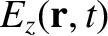
The previous equation determines the frequencies and polarizations of an electromagnetic
wave of wavenumber  that propagates through a magnetized plasma, and whose direction
of propagation subtends an angle with the magnetic field.
that propagates through a magnetized plasma, and whose direction
of propagation subtends an angle with the magnetic field.
Suppose, finally, that
It follows, from Equations (9.145)–(9.147), that
 ,
,
 , and
, and
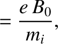
 . Hence, Equation (9.164) transforms to give the eigenmode equation
![\begin{displaymath}\left(
\begin{array}{ccc}
S-n^{\,2}\cos^2\theta,& D,&n^{\,2}\...
...ft(\begin{array}{c}0\\ [0.5ex] 0\\ [0.5ex] 0\end{array}\right).\end{displaymath}](img2817.png) |
(9.168) |
Here,
 |
(9.169) |
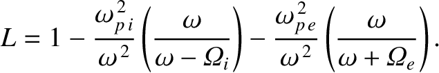
is the effective refractive index of the plasma, whereas


![$\displaystyle =-\epsilon_0\left[ \frac{\omega_{p\,i}^{\,2}}{\omega\,(\omega+{\mit\Omega}_i)}+\frac{\omega_{p\,e}^{\,2}}{\omega\,(\omega-{\mit\Omega}_e)}\right],$](img2748.png)