Pulse Propagation in Two Dimensions
In Section 6.10, we saw that a wave can propagate through an inhomogeneous medium, without significant reflection,
provided that the properties of the medium vary on lengthscales that are much longer than the wavelength of the wave. In
this section, we shall determine the path taken by a localized wave pulse as it travels though such a medium. For the sake of simplicity, we
shall restrict our analysis to two dimensions (by neglecting any variation in the  -direction.)
The wavefunction of a two-dimensional wave propagating through a (slowly varying) inhomogeneous medium can be written
in the general form
![$\displaystyle \psi(x,z,t) = A(x,z)\,\cos\left[\phi(x,z,t)\right].$](img2943.png) |
(9.230) |
Here,  is a relatively slowly varying function that determines the wave amplitude, whereas
 is a
relatively rapidly varying function that determines the wave phase. We can expand
locally as a
Taylor series (see Appendix B) to give
is a
relatively rapidly varying function that determines the wave phase. We can expand
locally as a
Taylor series (see Appendix B) to give
 |
(9.231) |
Comparison of the previous two equations with the standard expression for the wavefunction of a plane wave (see Section 7.2),
 |
(9.232) |
which is assumed to hold locally at each point in space, reveals that
where  is the wave angular frequency, and
 , 0,
, 0,  the wavevector. (The generalization to three dimensions is straightforward.)
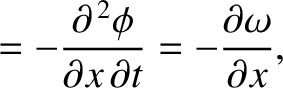
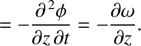
The previous three equations also imply that
the wavevector. (The generalization to three dimensions is straightforward.)
The previous three equations also imply that
As we saw in Section 9.2, a one-dimensional wave pulse propagating through a dispersive medium does so
at the group velocity,
 , where
 is the dispersion relation. Thus, the equation of motion
of the pulse is written
is the dispersion relation. Thus, the equation of motion
of the pulse is written
 |
(9.238) |
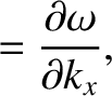
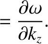
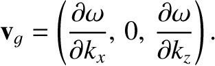
In two dimensions, the dispersion relation (in a uniform medium) takes the form
 . In this case, the
expression for the group velocity generalizes to (Landau and Lifshitz 1959)
. In this case, the
expression for the group velocity generalizes to (Landau and Lifshitz 1959)
 |
(9.239) |
(The generalization to three dimensions is straightforward.) Thus, in two dimensions, the equations of motion of a wave pulse are
It turns out that these equations also hold in a two-dimensional inhomogeneous medium; that is, a medium in which the
dispersion relation is an explicit function of position, so that
 . (Actually, this is only
true as long as the dispersion relation varies on lengthscales that are much longer than the wavelength.)
Thus, in a two-dimensional inhomogeneous medium, once we know the local dispersion relation,
,
we can trace the path of a wave pulse using the following four equations [cf., Equations (9.236)–(9.237) and (9.240)–(9.241)]:
(Incidentally,
. (Actually, this is only
true as long as the dispersion relation varies on lengthscales that are much longer than the wavelength.)
Thus, in a two-dimensional inhomogeneous medium, once we know the local dispersion relation,
,
we can trace the path of a wave pulse using the following four equations [cf., Equations (9.236)–(9.237) and (9.240)–(9.241)]:
(Incidentally,  ,
,  ,
,  , and
, and  are treated as independent variables in these equations.)
It can be seen that the preceding equations are analogous to Hamilton's equations for two-dimensional motion
in classical mechanics, with the wave vector playing the role of the momentum, and the function
are treated as independent variables in these equations.)
It can be seen that the preceding equations are analogous to Hamilton's equations for two-dimensional motion
in classical mechanics, with the wave vector playing the role of the momentum, and the function
 playing the role of the Hamiltonian (Goldstein, Poole, and Safko 2002). (In fact, Hamilton's equations were first derived to
determine the path of a light ray through an inhomogeneous medium, and only later applied to dynamical systems.)
playing the role of the Hamiltonian (Goldstein, Poole, and Safko 2002). (In fact, Hamilton's equations were first derived to
determine the path of a light ray through an inhomogeneous medium, and only later applied to dynamical systems.)
Consider a radio wave pulse launched from the Earth's surface, and subsequently reflected by the ionosphere. Let measure horizontal distance, and let
measure vertical height above the Earth's surface. Neglecting the Earth's weak magnetic field, the appropriate dispersion relation is (see Section 9.3)
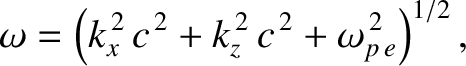 |
(9.246) |
where  is the velocity of light in vacuum, and
 the (electron) plasma frequency. This
frequency is proportional to the square root of the number density of free electrons in the
atmosphere, which we would generally expect to be a function of height only. In other words,
the (electron) plasma frequency. This
frequency is proportional to the square root of the number density of free electrons in the
atmosphere, which we would generally expect to be a function of height only. In other words,
 . Equations (9.242)–(9.244) yield
It is helpful to rewrite the dispersion relation as
. Equations (9.242)–(9.244) yield
It is helpful to rewrite the dispersion relation as
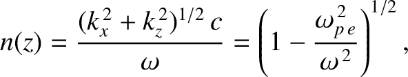 |
(9.250) |
where  is the refractive index.
Let us assume that  at
at  , which is equivalent to the reasonable assumption that the atmosphere
is non-ionized at ground level. It follows from Equation (9.249) that
, which is equivalent to the reasonable assumption that the atmosphere
is non-ionized at ground level. It follows from Equation (9.249) that
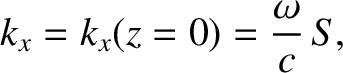 |
(9.251) |
where  is the sine of the angle of incidence of the pulse, with respect to the
vertical axis, at ground level. The previous two equations can be combined to give
is the sine of the angle of incidence of the pulse, with respect to the
vertical axis, at ground level. The previous two equations can be combined to give
 |
(9.252) |
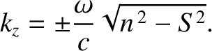
According to Equation (9.248), the plus sign corresponds to the upward trajectory of the pulse, whereas
the minus sign corresponds to the downward trajectory. Equations (9.247), (9.248), (9.251),
and (9.252) give the following equations of motion of the pulse:
It can be seen that the pulse attains its maximum altitude,  , when
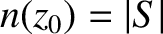 . The
total distance traveled by the pulse (i.e., the distance from its launch point to the point where it intersects the Earth's
surface again) is
. The
total distance traveled by the pulse (i.e., the distance from its launch point to the point where it intersects the Earth's
surface again) is
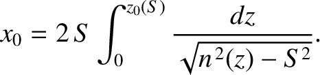 |
(9.255) |
According to Equations (9.247), (9.248), and (9.252), the equations of motion
of the pulse can also be written
It follows that the trajectory of the pulse is the same as that of a particle
moving in the gravitational potential
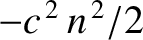 . In particular, if
  decreases linearly
with increasing altitude (as would be the case if the number density of free electrons
increased linearly with ) then the trajectory of the pulse is a parabola.
decreases linearly
with increasing altitude (as would be the case if the number density of free electrons
increased linearly with ) then the trajectory of the pulse is a parabola.