Three Spring-Coupled Masses
Consider a generalized version of the mechanical system discussed in Section 3.2
that consists of three identical masses  which slide over a
frictionless horizontal surface, and are connected by identical
light horizontal springs of spring constant
which slide over a
frictionless horizontal surface, and are connected by identical
light horizontal springs of spring constant  . As before, the outermost masses are attached to immovable
walls by springs of spring constant . The instantaneous configuration of
the system is specified by the horizontal displacements of the
three masses from their equilibrium positions; namely,
. As before, the outermost masses are attached to immovable
walls by springs of spring constant . The instantaneous configuration of
the system is specified by the horizontal displacements of the
three masses from their equilibrium positions; namely,  ,
,  , and
, and  .
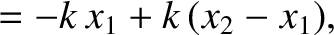
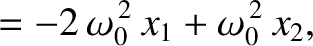
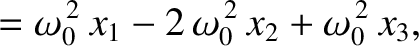
This is manifestly a three-degree-of-freedom system. We, therefore,
expect it to possess
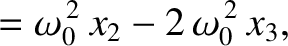
three independent normal modes of oscillation. Equations (3.1)–(3.2)
generalize to give
These equations can be rewritten
where
.
This is manifestly a three-degree-of-freedom system. We, therefore,
expect it to possess
three independent normal modes of oscillation. Equations (3.1)–(3.2)
generalize to give
These equations can be rewritten
where
 .
Let us search for a normal mode solution of the form
Equations (3.55)–(3.60) can be combined to give the
.
Let us search for a normal mode solution of the form
Equations (3.55)–(3.60) can be combined to give the  homogeneous matrix equation
![$\displaystyle \left(\begin{array}{ccc}
\hat{\omega}^{\,2}-2, & 1, & 0\\ [0.5ex]...
...ay}\right)
=\left(\begin{array}{c}0\\ [0.5ex] 0 \\ [0.5ex] 0\end{array}\right),$](img795.png) |
(3.61) |
where
 .
The normal frequencies are determined by setting the determinant of the matrix
to zero; that is,
.
The normal frequencies are determined by setting the determinant of the matrix
to zero; that is,
![$\displaystyle (\hat{\omega}^{\,2}-2)\left[(\hat{\omega}^{\,2}-2)^2-1\right]-(\hat{\omega}^{\,2}-2)=0,$](img796.png) |
(3.62) |
or
![$\displaystyle (\hat{\omega}^{\,2}-2)\,\left[\hat{\omega}^{\,2}-2-\sqrt{2}\right]\,\left[
\hat{\omega}^{\,2}-2+\sqrt{2}\right]=0.$](img797.png) |
(3.63) |
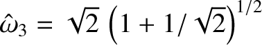
Thus, the normal frequencies are
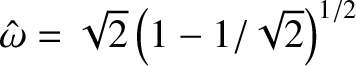 ,
,  , and
, and
 . According to the first and third rows
of Equation (3.61),
. According to the first and third rows
of Equation (3.61),
 |
(3.64) |
provided
 . According to the second row,
 |
(3.65) |
when
 .
Incidentally, we can only determine the ratios of
.
Incidentally, we can only determine the ratios of  ,
,  , and
, and
 , rather
than the absolute values of these quantities. In other words, only the direction of the vector
, rather
than the absolute values of these quantities. In other words, only the direction of the vector
 is well-defined. [This follows
because the most general solution, (3.69), is undetermined to an arbitrary multiplicative constant.
That is, if
is well-defined. [This follows
because the most general solution, (3.69), is undetermined to an arbitrary multiplicative constant.
That is, if
 is a solution to the dynamical equations (3.55)–(3.57) then so is
 , where
  is an arbitrary constant. This, in turn,
follows because the dynamical equations are linear.]
Let us
arbitrarily set the magnitude of
is an arbitrary constant. This, in turn,
follows because the dynamical equations are linear.]
Let us
arbitrarily set the magnitude of
 to unity. It follows that
the normal mode associated with the normal frequency
to unity. It follows that
the normal mode associated with the normal frequency
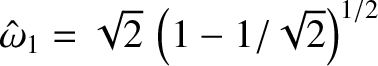 is
is
 |
(3.66) |
Likewise, the normal mode associated with the normal frequency
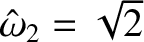 is
is
 |
(3.67) |
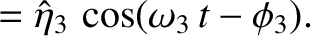
Finally, the
normal mode associated with the normal frequency
 is
is
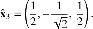 |
(3.68) |
Note that the vectors
 ,
,
 , and
, and
 are mutually perpendicular. In other words,
they are normal vectors. (Hence, the name “normal” mode.)
are mutually perpendicular. In other words,
they are normal vectors. (Hence, the name “normal” mode.)
Let
 . It follows that the most general solution to the problem is
 |
(3.69) |
where
Here,
 and
and
 are arbitrary constants. Incidentally, we need to introduce the arbitrary amplitudes
to make up for the fact that we set the magnitudes of the vectors
are arbitrary constants. Incidentally, we need to introduce the arbitrary amplitudes
to make up for the fact that we set the magnitudes of the vectors
 to unity.
Equation (3.69) yields
to unity.
Equation (3.69) yields
![$\displaystyle \left(\begin{array}{c}x_1\\ [0.5ex]x_2\\ [0.5ex]x_3\end{array}\ri...
...)\left(\begin{array}{c}\eta_1\\ [0.5ex]\eta_2\\ [0.5ex]\eta_3\end{array}\right)$](img827.png) |
(3.73) |
The preceding equation can be inverted by noting that
 , et cetera, because
,
,
and
are mutually perpendicular unit vectors. Thus, we obtain
, et cetera, because
,
,
and
are mutually perpendicular unit vectors. Thus, we obtain
![$\displaystyle \left(\begin{array}{c}\eta_1\\ [0.5ex]\eta_2\\ [0.5ex]\eta_3\end{...
...ay}\right)\left(\begin{array}{c}x_1\\ [0.5ex]x_2\\ [0.5ex]x_3\end{array}\right)$](img829.png) |
(3.74) |
This equation determines the three normal coordinates,  ,
,  ,
,  ,
in terms of the three physical coordinates,
,
in terms of the three physical coordinates,  ,
,  ,
,  . In general,
the normal coordinates are undetermined to arbitrary multiplicative constants.
. In general,
the normal coordinates are undetermined to arbitrary multiplicative constants.