Motion in a general 1-dimensional potential

Suppose that the curve $U(x)$ in Fig. 43 represents the potential energy of some mass $m$ moving in a 1-dimensional conservative force-field. For instance, $U(x)$ might represent the gravitational potential energy of a cyclist freewheeling in a hilly region. Note that we have set the potential energy at infinity to zero. This is a useful, and quite common, convention (recall that potential energy is undefined to within an arbitrary additive constant). What can we deduce about the motion of the mass in this potential?

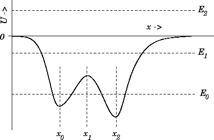
Figure 43: General 1-dimensional potential

Well, we know that the total energy, $E$--which is the sum of the kinetic energy, $K$, and the potential energy, $U$--is a constant of the motion. Hence, we can write

$$K(x) = E - U(x).$$ (170)

Now, we also know that a kinetic energy can never be negative, so the above expression tells us that the motion of the mass is restricted to the region (or regions) in which the potential energy curve $U(x)$ falls below the value $E$. This idea is illustrated in Fig. 43. Suppose that the total energy of the system is $E_0$. It is clear, from the figure, that the mass is trapped inside one or other of the two dips in the potential--these dips are generally referred to as potential wells. Suppose that we now raise the energy to $E_1$. In this case, the mass is free to enter or leave each of the potential wells, but its motion is still bounded to some extent, since it clearly cannot move off to infinity. Finally, let us raise the energy to $E_2$. Now the mass is unbounded: i.e., it can move off to infinity. In systems in which it makes sense to adopt the convention that the potential energy at infinity is zero, bounded systems are characterized by $E<0$, whereas unbounded systems are characterized by $E>0$.

The above discussion suggests that the motion of a mass moving in a potential generally becomes less bounded as the total energy $E$ of the system increases. Conversely, we would expect the motion to become more bounded as $E$ decreases. In fact, if the energy becomes sufficiently small, it appears likely that the system will settle down in some equilibrium state in which the mass is stationary. Let us try to identify any prospective equilibrium states in Fig. 43. 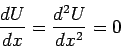If the mass remains stationary then it must be subject to zero force (otherwise it would accelerate). Hence, according to Eq. (164), an equilibrium state is characterized by

$$\frac{dU}{dx} = 0.$$ (171)

In other words, a equilibrium state corresponds to either a maximum or a minimum of the potential energy curve $U(x)$. It can be seen that the $U(x)$ curve shown in Fig. 43 has three associated equilibrium states: these are located at $x=x_0$, $x=x_1$, and $x=x_2$.

Let us now make a distinction between stable equilibrium points and unstable equilibrium points. When the system is slightly perturbed from a stable equilibrium point then the resultant force $f$ should always be such as to attempt to return the system to this point. In other words, if $x=x_0$ is an equilibrium point, then we require

$$\left.\frac{df}{dx}\right\vert _{x_0} <0$$ (172)

for stability: i.e., if the system is perturbed to the right, so that $x-x_0>0$, then the force must act to the left, so that $f <0$, and vice versa. Likewise, if

$$\left.\frac{df}{dx}\right\vert _{x_0} >0$$ (173)

then the equilibrium point $x=x_0$ is unstable. It follows, from Eq. (164), that stable equilibrium points are characterized by

$$\frac{d^2 U}{dx^2}>0.$$ (174)

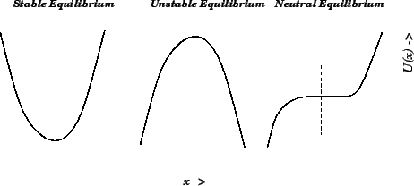
In other words, a stable equilibrium point corresponds to a minimum of the potential energy curve $U(x)$. Likewise, an unstable equilibrium point corresponds to a maximum of the $U(x)$ curve. Hence, we conclude that $x=x_0$ and $x=x_2$ are stable equilibrium points, in Fig. 43, whereas $x=x_1$ is an unstable equilibrium point. Of course, this makes perfect sense if we think of $U(x)$ as a gravitational potential energy curve, in which case $U$ is directly proportional to height. All we are saying is that it is easy to confine a low energy mass at the bottom of a valley, but very difficult to balance the same mass on the top of a hill (since any slight perturbation to the mass will cause it to fall down the hill). Note, finally, that if

$$\frac{dU}{dx}=\frac{d^2 U}{dx^2}=0$$ (175)

at any point (or in any region) then we have what is known as a neutral equilibrium point. We can move the mass slightly off such a point and it will still remain in equilibrium (i.e., it will neither attempt to return to its initial state, nor will it continue to move). A neutral equilibrium point corresponds to a flat spot in a $U(x)$ curve. See Fig. 44.

Figure 44: Different types of equilibrium