The simple pendulum

Consider a mass $m$ suspended from a light inextensible string of length $l$, such that the mass is free to swing from side to side in a vertical plane, as shown in Fig. 97. This setup is known as a simple pendulum. Let $\theta$ be the angle subtended between the string and the downward vertical. Obviously, the equilibrium state of the simple pendulum corresponds to the situation in which the mass is stationary and hanging vertically down (i.e., $\theta=0$). The angular equation of motion of the pendulum is simply

$$I \ddot{\theta} = \tau,$$ (523)

where $I$ is the moment of inertia of the mass, and $\tau$ is the torque acting on the system. For the case in hand, given that the mass is essentially a point particle, and is situated a distance $l$ from the axis of rotation (i.e., the pivot point), it is easily seen that $I=m l^2$.

Figure 97: A simple pendulum.

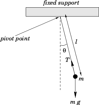The two forces acting on the mass are the downward gravitational force, $m g$, and the tension, $T$, in the string. Note, however, that the tension makes no contribution to the torque, since its line of action clearly passes through the pivot point. From simple trigonometry, the line of action of the gravitational force passes a distance $l \sin\theta$ from the pivot point. Hence, the magnitude of the gravitational torque is $m g l \sin\theta$. Moreover, the gravitational torque is a restoring torque: i.e., if the mass is displaced slightly from its equilibrium state (i.e., $\theta=0$) then the gravitational force clearly acts to push the mass back toward that state. Thus, we can write

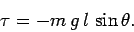$$\tau = - m g l \sin\theta.$$ (524)

Combining the previous two equations, we obtain the following angular equation of motion of the pendulum:

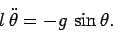$$l \ddot{\theta} = - g \sin\theta.$$ (525)

Unfortunately, this is not the simple harmonic equation. Indeed, the above equation possesses no closed solution which can be expressed in terms of simple functions.

Suppose that we restrict our attention to relatively small deviations from the equilibrium state. In other words, suppose that the angle $\theta$ is constrained to take fairly small values. We know, from trigonometry, that for $\vert\theta\vert$ less than about $6^\circ$ it is a good approximation to write

$$\sin\theta \simeq \theta.$$ (526)

Hence, in the small angle limit, Eq. (525) reduces to

$$l \ddot{\theta} = - g \theta,$$ (527)

which is in the familiar form of a simple harmonic equation. Comparing with our original simple harmonic equation, Eq. (504), and its solution, we conclude that the angular frequency of small amplitude oscillations of a simple pendulum is given by

$$\omega = \sqrt{\frac{g}{l}}.$$ (528)

In this case, the pendulum frequency is dependent only on the length of the pendulum and the local gravitational acceleration, and is independent of the mass of the pendulum and the amplitude of the pendulum swings (provided that $\sin\theta \simeq \theta$ remains a good approximation). Historically, the simple pendulum was the basis of virtually all accurate time-keeping devices before the advent of electronic clocks. Simple pendulums can also be used to measure local variations in $g$.