Paramagnetism

The simplest microscopic system which we can analyze using the Boltzmann distribution is one which has only two possible states (there would clearly be little point in analyzing a system with only one possible state). Most elements, and some compounds, are paramagnetic: i.e., their constituent atoms, or molecules, possess a permanent magnetic moment due to the presence of one or more unpaired electrons. Consider a substance whose constituent particles contain only one unpaired electron. Such particles have spin $1/2$, and consequently possess an intrinsic magnetic moment $\mu$. According to quantum mechanics, the magnetic moment of a spin $1/2$ particle can point either parallel or antiparallel to an external magnetic field ${\bf B}$. Let us determine the mean magnetic moment $\overline{\mu}_B$ (in the direction of ${\bf B}$) of the constituent particles of the substance when its absolute temperature is $T$. We assume, for the sake of simplicity, that each atom (or molecule) only interacts weakly with its neighbouring atoms. This enables us to focus attention on a single atom, and treat the remaining atoms as a heat bath at temperature $T$.

Our atom can be in one of two possible states: the $(+)$ state in which its spin points up (i.e., parallel to ${\bf B}$), and the $(-)$ state in which its spin points down (i.e., antiparallel to ${\bf B}$). In the $(+)$ state, the atomic magnetic moment is parallel to the magnetic field, so that $\mu_B = \mu$. The magnetic energy of the atom is $\epsilon_{+} = - \mu \, B$. In the $(-)$ state, the atomic magnetic moment is antiparallel to the magnetic field, so that $\mu_B = -\mu$. The magnetic energy of the atom is $\epsilon_{-} = \mu \, B$.

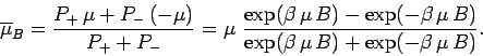
According to the Boltzmann distribution, the probability of finding the atom in the $(+)$ state is

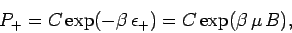$$P_{+} = C\exp(-\beta\,\epsilon_{+}) = C\exp(\beta\, \mu \,B),$$ (381)

where $C$ is a constant, and $\beta = (k\,T)^{-1}$. Likewise, the probability of finding the atom in the $(-)$ state is

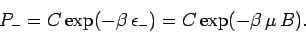$$P_{-} = C\exp(-\beta\,\epsilon_{-}) = C\exp(-\beta\, \mu\, B).$$ (382)

Clearly, the most probable state is the state with the lowest energy [i.e., the $(+)$ state]. Thus, the mean magnetic moment points in the direction of the magnetic field (i.e., the atom is more likely to point parallel to the field than antiparallel).

It is clear that the critical parameter in a paramagnetic system is

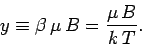$$y\equiv \beta\,\mu \,B = \frac{\mu \,B}{k\,T}.$$ (383)

This parameter measures the ratio of the typical magnetic energy of the atom to its typical thermal energy. If the thermal energy greatly exceeds the magnetic energy then $y\ll 1$, and the probability that the atomic moment points parallel to the magnetic field is about the same as the probability that it points antiparallel. In this situation, we expect the mean atomic moment to be small, so that $\overline{\mu}_B \simeq 0$. On the other hand, if the magnetic energy greatly exceeds the thermal energy then $y\gg 1$, and the atomic moment is far more likely to point parallel to the magnetic field than antiparallel. In this situation, we expect $\overline{\mu}_B\simeq \mu$.

Let us calculate the mean atomic moment $\overline{\mu}_B$. The usual definition of a mean value gives

$$\overline{\mu}_B = \frac{ P_{+}\, \mu + P_{-} \,(-\mu)}{P_{+... ... \,\mu \,B)} { \exp(\beta \,\mu \,B)+ \exp(-\beta \,\mu \,B)}.$$ (384)

This can also be written

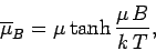$$\overline{\mu}_B = \mu \tanh\frac{\mu\, B}{k\,T},$$ (385)

where the hyperbolic tangent is defined

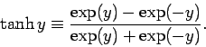$$\tanh y \equiv \frac{ \exp(y) - \exp(-y)}{\exp(y)+\exp(-y)}.$$ (386)

For small arguments, $y\ll 1$,

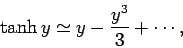$$\tanh y \simeq y - \frac{y^3}{3} +\cdots,$$ (387)

whereas for large arguments, $y\gg 1$,

$$\tanh y \simeq 1.$$ (388)

It follows that at comparatively high temperatures, $k\, T\gg \mu \,B$,

$$\overline{\mu}_B \simeq \frac{\mu^2 B}{k\,T},$$ (389)

whereas at comparatively low temperatures, $k \,T \ll \mu\, B$,

$$\overline{\mu}_B \simeq \mu.$$ (390)

Suppose that the substance contains $N_0$ atoms (or molecules) per unit volume. The magnetization is defined as the mean magnetic moment per unit volume, and is given by

$$\overline{M}_0 = N_0\, \overline{\mu}_B.$$ (391)

At high temperatures, $k\, T\gg \mu \,B$, the mean magnetic moment, and, hence, the magnetization, is proportional to the applied magnetic field, so we can write

$$\overline{M}_0 \simeq \chi\, B,$$ (392)

where $\chi$ is a constant of proportionality known as the magnetic susceptibility. It is clear that the magnetic susceptibility of a spin 1/2 paramagnetic substance takes the form

$$\chi = \frac{N_0\, \mu^2}{k\,T}.$$ (393)

The fact that $\chi\propto T^{-1}$ is known as Curie's law, because it was discovered experimentally by Pierre Curie at the end of the nineteenth century. At low temperatures, $k \,T \ll \mu\, B$,

$$\overline{M}_0 \rightarrow N_0 \,\mu,$$ (394)

so the magnetization becomes independent of the applied field. This corresponds to the maximum possible magnetization, where all atomic moments are lined up parallel to the field. The breakdown of the $\overline{M}_0 \propto B$ law at low temperatures (or high magnetic fields) is known as saturation.

Figure 2: The magnetization (vertical axis) versus $B/T$ (horizontal axis) curves for (I) chromium potassium alum ($J=3/2$), (II) iron ammonium alum ($J=5/2$), and (III) gadolinium sulphate ($J=7/2$). The solid lines are the theoretical predictions whereas the data points are experimental measurements. From W.E. Henry, Phys. Rev. 88, 561 (1952).

The above analysis is only valid for paramagnetic substances made up of spin one-half ($J=1/2$) atoms or molecules. However, the analysis can easily be generalized to take account of substances whose constituent particles possess higher spin (i.e., $J>1/2$). Figure 2 compares the experimental and theoretical magnetization versus field-strength curves for three different substances made up of spin $3/2$, spin $5/2$, and spin $7/2$ particles, showing the excellent agreement between the two sets of curves. Note that, in all cases, the magnetization is proportional to the magnetic field-strength at small field-strengths, but saturates at some constant value as the field-strength increases.

The previous analysis completely neglects any interaction between the spins of neighbouring atoms or molecules. It turns out that this is a fairly good approximation for paramagnetic substances. However, for ferromagnetic substances, in which the spins of neighbouring atoms interact very strongly, this approximation breaks down completely. Thus, the above analysis does not apply to ferromagnetic substances.