Boltzmann distributions

We have gained some understanding of the macroscopic properties of the air around us. For instance, we know something about its internal energy and specific heat capacity. How can we obtain some information about the statistical properties of the molecules which make up air? Consider a specific molecule: it constantly collides with its immediate neighbour molecules, and occasionally bounces off the walls of the room. These interactions ``inform'' it about the macroscopic state of the air, such as its temperature, pressure, and volume. The statistical distribution of the molecule over its own particular microstates must be consistent with this macrostate. In other words, if we have a large group of such molecules with similar statistical distributions, then they must be equivalent to air with the appropriate macroscopic properties. So, it ought to be possible to calculate the probability distribution of the molecule over its microstates from a knowledge of these macroscopic properties.

We can think of the interaction of a molecule with the air in a classroom as analogous to the interaction of a small system $A$ in thermal contact with a heat reservoir $A'$. The air acts like a heat reservoir because its energy fluctuations due to any interactions with the molecule are far too small to affect any of its macroscopic parameters. Let us determine the probability $P_r$ of finding system $A$ in one particular microstate $r$ of energy $E_r$ when it is thermal equilibrium with the heat reservoir $A'$.

As usual, we assume fairly weak interaction between $A$ and $A'$, so that the energies of these two systems are additive. The energy of $A$ is not known at this stage. In fact, only the total energy of the combined system $A^{(0)} = A + A'$ is known. Suppose that the total energy lies in the range $E^{(0)}$ to $E^{(0)} + \delta E$. The overall energy is constant in time, since $A^{(0)}$ is assumed to be an isolated system, so

$$E_r + E' = E^{(0)},$$ (369)

where $E'$ denotes the energy of the reservoir $A'$. Let ${\mit\Omega}'(E')$ be the number of microstates accessible to the reservoir when its energy lies in the range $E'$ to $E'+\delta E$. Clearly, if system $A$ has an energy $E_r$ then the reservoir $A'$ must have an energy close to $E'=E^{(0)} - E_r$. Hence, since $A$ is in one definite state (i.e., state $r$), and the total number of states accessible to $A'$ is ${\mit\Omega}'(E^{(0)} - E_r)$, it follows that the total number of states accessible to the combined system is simply ${\mit\Omega}'(E^{(0)} - E_r)$. The principle of equal a priori probabilities tells us the the probability of occurrence of a particular situation is proportional to the number of accessible microstates. Thus,

$$P_r = C' \,{\mit\Omega}'(E^{(0)} - E_r),$$ (370)

where $C'$ is a constant of proportionality which is independent of $r$. This constant can be determined by the normalization condition

$$\sum_r P_r = 1,$$ (371)

where the sum is over all possible states of system $A$, irrespective of their energy.

Let us now make use of the fact that system $A$ is far smaller than system $A'$. It follows that $E_r\ll E^{(0)}$, so the slowly varying logarithm of $P_r$ can be Taylor expanded about $E' = E^{(0)}$. Thus,

$$\ln P_r = \ln C' +\ln {\mit\Omega}'(E^{(0)}) -\left[\frac{\partial \ln {\mit\Omega}'} {\partial E'} \right]_0 E_r +\cdots.$$ (372)

Note that we must expand $\ln P_r$, rather than $P_r$ itself, because the latter function varies so rapidly with energy that the radius of convergence of its Taylor series is far too small for the series to be of any practical use. The higher order terms in Eq. (372) can be safely neglected, because $E_r\ll E^{(0)}$. Now the derivative

$$\left[\frac{\partial \ln {\mit\Omega}'}{\partial E'} \right]_0 \equiv \beta$$ (373)

is evaluated at the fixed energy $E' = E^{(0)}$, and is, thus, a constant independent of the energy $E_r$ of $A$. In fact, we know, from Sect. 5, that this derivative is just the temperature parameter $\beta = (k\,T)^{-1}$ characterizing the heat reservoir $A'$. Hence, Eq. (372) becomes

$$\ln P_r = \ln C' + \ln {\mit\Omega}'(E^{(0)}) - \beta\, E_r,$$ (374)

giving

$$P_r = C \exp(-\beta \,E_r),$$ (375)

where $C$ is a constant independent of $r$. The parameter $C$ is determined by the normalization condition, which gives

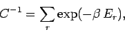$$C^{-1} = \sum_r \exp(-\beta \,E_r),$$ (376)

so that the distribution becomes

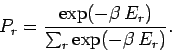$$P_r = \frac{\exp(-\beta\, E_r)}{\sum_r \exp(-\beta \,E_r)}.$$ (377)

This is known as the Boltzmann probability distribution, and is undoubtably the most famous result in statistical physics.

The Boltzmann distribution often causes confusion. People who are used to the principle of equal a priori probabilities, which says that all microstates are equally probable, are understandably surprised when they come across the Boltzmann distribution which says that high energy microstates are markedly less probable then low energy states. However, there is no need for any confusion. The principle of equal a priori probabilities applies to the whole system, whereas the Boltzmann distribution only applies to a small part of the system. The two results are perfectly consistent. If the small system is in a microstate with a comparatively high energy $E_r$ then the rest of the system (i.e., the reservoir) has a slightly lower energy $E'$ than usual (since the overall energy is fixed). The number of accessible microstates of the reservoir is a very strongly increasing function of its energy. It follows that when the small system has a high energy then significantly less states than usual are accessible to the reservoir, and so the number of microstates accessible to the overall system is reduced, and, hence, the configuration is comparatively unlikely. The strong increase in the number of accessible microstates of the reservoir with increasing $E'$ gives rise to the strong (i.e., exponential) decrease in the likelihood of a state $r$ of the small system with increasing $E_r$. The exponential factor $\exp(-\beta \,E_r)$ is called the Boltzmann factor.

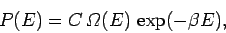
The Boltzmann distribution gives the probability of finding the small system $A$ in one particular state $r$ of energy $E_r$. The probability $P(E)$ that $A$ has an energy in the small range between $E$ and $E+\delta E$ is just the sum of all the probabilities of the states which lie in this range. However, since each of these states has approximately the same Boltzmann factor this sum can be written

$$P(E) = C \,{\mit\Omega}(E)\,\exp(-\beta E),$$ (378)

where ${\mit\Omega}(E)$ is the number of microstates of $A$ whose energies lie in the appropriate range. Suppose that system $A$ is itself a large system, but still very much smaller than system $A'$. For a large system, we expect ${\mit\Omega}(E)$ to be a very rapidly increasing function of energy, so the probability $P(E)$ is the product of a rapidly increasing function of $E$ and another rapidly decreasing function (i.e., the Boltzmann factor). This gives a sharp maximum of $P(E)$ at some particular value of the energy. The larger system $A$, the sharper this maximum becomes. Eventually, the maximum becomes so sharp that the energy of system $A$ is almost bound to lie at the most probable energy. As usual, the most probable energy is evaluated by looking for the maximum of $\ln P$, so

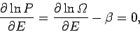$$\frac{\partial \ln P}{\partial E} = \frac{\partial \ln {\mit\Omega}}{\partial E} -\beta =0,$$ (379)

giving

$$\frac{\partial \ln {\mit\Omega}}{\partial E} = \beta.$$ (380)

Of course, this corresponds to the situation in which the temperature of $A$ is the same as that of the reservoir. This is a result which we have seen before (see Sect. 5). Note, however, that the Boltzmann distribution is applicable no matter how small system $A$ is, so it is a far more general result than any we have previously obtained.