Next: Temperature
Up: Statistical thermodynamics
Previous: Introduction
Thermal interaction between macrosystems
Let us begin our investigation of statistical thermodynamics
by examining
a purely thermal interaction between two macroscopic
systems,  and
and  , from a microscopic point of view. Suppose that the energies of
these two systems are
, from a microscopic point of view. Suppose that the energies of
these two systems are  and
and  , respectively. The external parameters are held
fixed, so that and cannot do work on one another. However, we
assume that
the systems are free to exchange heat energy (i.e., they are in thermal contact).
It is convenient to divide the energy
scale into small subdivisions of width
, respectively. The external parameters are held
fixed, so that and cannot do work on one another. However, we
assume that
the systems are free to exchange heat energy (i.e., they are in thermal contact).
It is convenient to divide the energy
scale into small subdivisions of width  .
The number of microstates of consistent with a
macrostate in which the energy lies in the range to
.
The number of microstates of consistent with a
macrostate in which the energy lies in the range to  is denoted
 . Likewise, the number of microstates of consistent with a
macrostate in which the energy lies between and
. Likewise, the number of microstates of consistent with a
macrostate in which the energy lies between and  is
denoted
is
denoted
 .
.
The combined system
 is assumed to be
isolated (i.e., it neither does work on
nor exchanges heat with its surroundings). It follows from the first law of
thermodynamics that the total energy
is assumed to be
isolated (i.e., it neither does work on
nor exchanges heat with its surroundings). It follows from the first law of
thermodynamics that the total energy  is constant.
When
speaking of thermal contact between two distinct
systems, we usually assume that the mutual interaction is
sufficiently weak for the energies to be additive. Thus,
is constant.
When
speaking of thermal contact between two distinct
systems, we usually assume that the mutual interaction is
sufficiently weak for the energies to be additive. Thus,
 |
(157) |
Of course, in the limit of zero
interaction the energies are strictly additive. However,
a small residual interaction is always required to enable the two systems to exchange
heat energy and, thereby, eventually
reach thermal equilibrium (see Sect. 3.4). In fact, if
the interaction between and is too strong for the energies to be
additive then it makes little
sense to consider each system in isolation, since the presence of one system clearly
strongly perturbs the other, and vice versa. In this case, the smallest system
which can realistically be examined in isolation is  .
.
According to Eq. (157), if the energy of lies in the range to
then the energy of must lie between
 and
and  .
Thus, the number of microstates accessible to each system is
given by
and
.
Thus, the number of microstates accessible to each system is
given by
and
 , respectively.
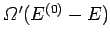
Since every possible state of can be
combined with every possible state of to form a distinct microstate,
the total number of distinct states
accessible to when the energy of lies in the range to
is
, respectively.
Since every possible state of can be
combined with every possible state of to form a distinct microstate,
the total number of distinct states
accessible to when the energy of lies in the range to
is
 |
(158) |
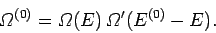
Consider an ensemble of pairs of thermally interacting systems,
and , which are left undisturbed
for many relaxation times so that they can attain thermal equilibrium.
The principle of equal a priori probabilities is applicable to
this situation (see Sect. 3).
According to this principle, the probability of occurrence of a given macrostate
is proportional to the number of accessible microstates, since all microstates are
equally likely. Thus, the probability that the system has an energy lying in
the range to can be written
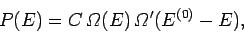 |
(159) |
where  is a constant which is independent of .
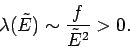
We know, from Sect. 3.8, that the typical variation of the number of accessible
states with energy is of the form
 |
(160) |
where  is the number of degrees of freedom. For a macroscopic system is
an exceedingly large number. It follows that the probability
is the number of degrees of freedom. For a macroscopic system is
an exceedingly large number. It follows that the probability
 in Eq. (159) is the product
of an extremely rapidly increasing function of
and an extremely rapidly decreasing
function of . Hence, we would expect the probability
to exhibit a very pronounced
maximum at some particular value of the energy.
in Eq. (159) is the product
of an extremely rapidly increasing function of
and an extremely rapidly decreasing
function of . Hence, we would expect the probability
to exhibit a very pronounced
maximum at some particular value of the energy.
Let us
Taylor expand the logarithm of in the vicinity of its maximum value, which
is assumed to occur at  . We expand the relatively slowly varying
logarithm, rather than the function itself, because the latter varies so rapidly
with the energy that the radius of convergence of its Taylor expansion
is too small for this expansion to be of any practical use.
The expansion of
. We expand the relatively slowly varying
logarithm, rather than the function itself, because the latter varies so rapidly
with the energy that the radius of convergence of its Taylor expansion
is too small for this expansion to be of any practical use.
The expansion of
 yields
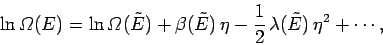 |
(161) |
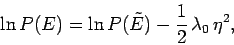
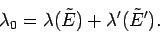
where
Now, since
 , we have
 |
(165) |
It follows that
 |
(166) |
where  and
and  are defined in an analogous manner to the parameters
 and
and  .
Equations (161) and (166) can be combined to give
.
Equations (161) and (166) can be combined to give
![\begin{displaymath}
\ln\,[{\mit\Omega}(E)\,{\mit\Omega}'(E')] = \ln\,[{\mit\Omeg...
...2}\,
[\lambda(\tilde{E})+\lambda'(\tilde{E}')]\,\eta^2+\cdots.
\end{displaymath}](img485.png) |
(167) |
At the maximum of
![$\ln\,[{\mit\Omega}(E) \,{\mit\Omega}'(E')]$](img486.png) the linear term in
the Taylor expansion must vanish, so
the linear term in
the Taylor expansion must vanish, so
 |
(168) |
which enables us to determine  . It follows that
 |
(169) |
or
![\begin{displaymath}
P(E)=P(\tilde{E}) \exp\left[-\frac{1}{2}\,\lambda_0\, (E-\tilde{E})^2\right],
\end{displaymath}](img490.png) |
(170) |
where
 |
(171) |
Now, the parameter  must be positive, otherwise the probability
does not exhibit a pronounced maximum value: i.e., the combined system
does not possess a well-defined equilibrium state as, physically, we know it must.
It is clear that
must be positive, otherwise the probability
does not exhibit a pronounced maximum value: i.e., the combined system
does not possess a well-defined equilibrium state as, physically, we know it must.
It is clear that
 must also be
positive, since we could always choose for a system with a negligible contribution
to , in which case the constraint
must also be
positive, since we could always choose for a system with a negligible contribution
to , in which case the constraint  would
effectively correspond to
would
effectively correspond to
 . [A similar argument can be used to
show that
. [A similar argument can be used to
show that
 must be
positive.] The same conclusion also follows from
the estimate
must be
positive.] The same conclusion also follows from
the estimate
 , which implies that
 |
(172) |
According to Eq. (170), the probability distribution function is
a Gaussian. This is hardly surprising, since the central limit theorem ensures that
the probability distribution for any macroscopic variable, such as , is Gaussian
in
nature (see Sect. 2.10). It follows that the mean value of corresponds to
the situation of maximum probability (i.e., the peak of the Gaussian curve), so
that
 |
(173) |
The standard deviation of the distribution is
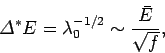 |
(174) |
where use has been made of Eq. (160) (assuming that system makes the dominant
contribution to ). It follows that the fractional width of the
probability distribution function is given by
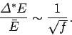 |
(175) |
Hence, if contains 1 mole of particles then
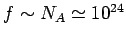 and
and
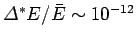 . Clearly, the probability
distribution for has an exceedingly sharp maximum. Experimental
measurements of this energy will almost always yield the mean value,
and the underlying
statistical nature of the distribution may not be apparent.
. Clearly, the probability
distribution for has an exceedingly sharp maximum. Experimental
measurements of this energy will almost always yield the mean value,
and the underlying
statistical nature of the distribution may not be apparent.
Next: Temperature
Up: Statistical thermodynamics
Previous: Introduction
Richard Fitzpatrick
2006-02-02