Next: Electric Dipole Approximation
Up: Time-Dependent Perturbation Theory
Previous: Harmonic Perturbations
Let us use the above results to investigate the interaction of an atomic electron with
classical (i.e., non-quantized) electromagnetic radiation.
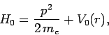
The unperturbed Hamiltonian of the system
is
 |
(1080) |
Now, the standard classical prescription for obtaining the Hamiltonian of
a particle
of charge  in the presence of an electromagnetic field is
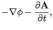
where
 is the vector potential, and
  the scalar potential. Note that
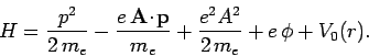
This prescription also works in quantum mechanics. Thus, the Hamiltonian
of an atomic electron placed in an electromagnetic field is
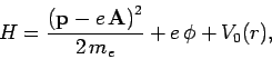 |
(1085) |
where  and
and  are functions of the position operators.
The above equation can be written
are functions of the position operators.
The above equation can be written
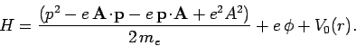 |
(1086) |
Now,
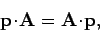 |
(1087) |
provided that we adopt the gauge
 .
Hence,
.
Hence,
 |
(1088) |
Suppose that the perturbation corresponds to a linearly polarized, monochromatic, plane-wave. In this case,
where  is the wavevector (note that
  ), and
 a unit vector which specifies the direction of polarization (i.e., the direction of
  ).
Note that
).
Note that
 . The Hamiltonian
becomes
. The Hamiltonian
becomes
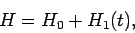 |
(1091) |
with
 |
(1092) |
and
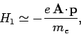 |
(1093) |
where the  term, which is second order in
  , has been neglected.
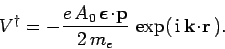
The perturbing Hamiltonian can be written
![\begin{displaymath}
H_1 = - \frac{e A_0 \mbox{\boldmath$\epsilon$}\!\cdot\!{...
...{\rm i} {\bf k}\!\cdot\!{\bf r} + {\rm i}
\omega t)\right].
\end{displaymath}](img2548.png) |
(1094) |
This has the same form as Eq. (1067), provided that
 |
(1095) |
It follows from Eqs. (1069), (1079), and (1095)
that the transition probability for radiation induced absorption is
![\begin{displaymath}
P_{i\rightarrow f}^{abs}(t) = \frac{t^2}{\hbar^2} \frac{e^2...
...gle\right\vert^{ 2} {\rm sinc}^2[(\omega-\omega_{fi}) t/2].
\end{displaymath}](img2550.png) |
(1096) |
Now, the mean energy density of an electromagnetic wave is
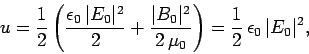 |
(1097) |
where
 and
and  are the peak electric
and magnetic field-strengths, respectively. It thus follows that
are the peak electric
and magnetic field-strengths, respectively. It thus follows that
![\begin{displaymath}
P_{i\rightarrow f}^{abs}(t) = \frac{t^2 e^2}{2 \epsilon_0\...
...\right\vert^{ 2} u {\rm sinc}^2[(\omega-\omega_{fi}) t/2].
\end{displaymath}](img2554.png) |
(1098) |
Thus, not surprisingly, the transition probability for radiation induced absorption (or stimulated emission) is directly proportional to the energy
density of the incident radiation.
Suppose that the incident radiation is not monochromatic, but instead
extends over a range of frequencies. We can write
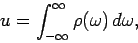 |
(1099) |
where
 is the energy density of radiation whose frequencies lie between
  and
and
 .
Equation (1098) generalizes to
.
Equation (1098) generalizes to
![\begin{displaymath}
P_{i\rightarrow f}^{abs}(t) = \int_{-\infty}^\infty\frac{t^2...
...rho(\omega) {\rm sinc}^2[(\omega-\omega_{fi}) t/2] d\omega.
\end{displaymath}](img2558.png) |
(1100) |
Note, however, that the above expression is only valid provided the radiation
in question is incoherent: i.e., there are no phase correlations between
waves of different frequencies. This follows because it is permissible to add the
intensities of incoherent radiation, whereas we must always add the
amplitudes of coherent radiation.
Given that the function
![${\rm sinc}^2[(\omega-\omega_{fi}) t/2]$](img2559.png) is very strongly peaked (see Fig. 25) about
is very strongly peaked (see Fig. 25) about
 (assuming that
 ), and
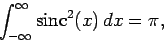 |
(1101) |
the above equation reduces to
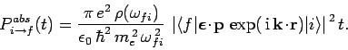 |
(1102) |
Note that in integrating over the frequencies of
the incoherent radiation we have transformed a transition
probability which is basically proportional to  [see Eq. (1098)] to one which is proportional to
  . As has
already been explained, the above expression is only valid when
. As has
already been explained, the above expression is only valid when
 . However, the result that
 |
(1103) |
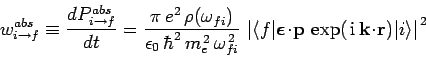
is constant in time is universally valid. Here,
 is the transition probability per unit time interval, otherwise known
as the transition rate. Given that the transition rate is constant,
we can write (see Cha. 2)
is the transition probability per unit time interval, otherwise known
as the transition rate. Given that the transition rate is constant,
we can write (see Cha. 2)
![\begin{displaymath}
P_{i\rightarrow f}^{abs}(t+dt) - P_{i\rightarrow f}^{abs}(t)...
...i\rightarrow f}^{abs}(t)\right] w_{i\rightarrow f}^{abs} dt:
\end{displaymath}](img2566.png) |
(1104) |
i.e., the probability that the system makes a transition from state
 to state
  between times and
  is equivalent to the probability that the
system does not make a transition between times 0 and and then makes
a transition in a time interval
is equivalent to the probability that the
system does not make a transition between times 0 and and then makes
a transition in a time interval  --the probabilities of these two events are
 and
and
 ,
respectively. It follows that
,
respectively. It follows that
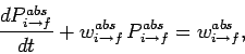 |
(1105) |
with the initial condition
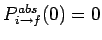 . The
above equation can be solved to give
. The
above equation can be solved to give
 |
(1106) |
This result is consistent with Eq. (1102) provided
 : i.e., provided
that
: i.e., provided
that
 .
.
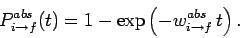
Using similar arguments to the above, the transition probability for
stimulated emission can be shown to take the form
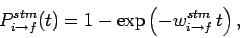 |
(1107) |
where the corresponding transition rate is written
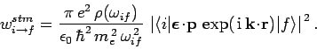 |
(1108) |
Next: Electric Dipole Approximation
Up: Time-Dependent Perturbation Theory
Previous: Harmonic Perturbations
Richard Fitzpatrick
2010-07-20