Next: Time-Dependent Perturbation Theory
Up: Time-Independent Perturbation Theory
Previous: Hyperfine Structure
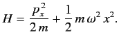
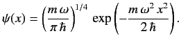
- Calculate the energy-shift in the ground state of the one-dimensional harmonic
oscillator when the perturbation
is added to
The properly normalized ground-state wavefunction is
- Calculate the energy-shifts due to the first-order Stark effect in the
 state of a hydrogen atom. You do not
need to perform all of the integrals, but you should construct the correct linear combinations of states.
state of a hydrogen atom. You do not
need to perform all of the integrals, but you should construct the correct linear combinations of states.
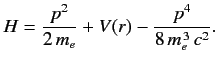
- The Hamiltonian of the valence electron in a hydrogen-like atom can be written
Here, the final term on the right-hand side is the first-order correction due to the electron's relativistic mass
increase. Treating this term as a small perturbation, deduce that it causes an energy-shift in the energy eigenstate
characterized by the standard quantum numbers  ,
,  ,
,  of
of
where  is the unperturbed energy, and
  the fine structure constant.
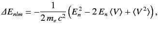
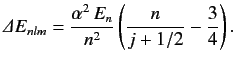
- Consider an energy eigenstate of the hydrogen atom characterized by the standard quantum numbers
,
, and
.
Show that if the energy-shift due to spin-orbit coupling (see Section 7.7) is added to that due to the electron's relativistic mass increase (see previous exercise) then the
net fine structure energy-shift can be written
Here,
is the unperturbed energy,
the fine structure constant, and
 the quantum number associated
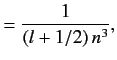
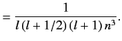
with the magnitude of the sum of the electron's orbital and spin angular momenta. You will need to use the following standard results for a hydrogen atom:
the quantum number associated
with the magnitude of the sum of the electron's orbital and spin angular momenta. You will need to use the following standard results for a hydrogen atom:
Here,  is the Bohr radius.
Assuming that the above formula for the energy shift is valid for
is the Bohr radius.
Assuming that the above formula for the energy shift is valid for  (which it is), show that fine structure causes the
energy of the
(which it is), show that fine structure causes the
energy of the
 states of a hydrogen atom to exceed those of the
 and
and
 states by
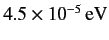 .
.
Next: Time-Dependent Perturbation Theory
Up: Time-Independent Perturbation Theory
Previous: Hyperfine Structure
Richard Fitzpatrick
2013-04-08