Next: Quadratic Stark Effect Up: Time-Independent Perturbation Theory Previous: Two-State System

Non-Degenerate Perturbation Theory

Let us now generalize our perturbation analysis to deal with systems possessing more than two energy eigenstates. The energy eigenstates of the unperturbed Hamiltonian, , are denoted

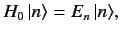$\displaystyle H_0\, \vert n\rangle = E_n\, \vert n\rangle,$

(601)

where runs from 1 to . The eigenkets $\vert n\rangle$ are orthogonal, form a complete set, and have their lengths normalized to unity. Let us now try to solve the energy eigenvalue problem for the perturbed Hamiltonian:

$\displaystyle (H_0 + H_1) \,\vert E\rangle = E\,\vert E\rangle.$

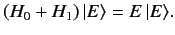(602)

We can express $\vert E\rangle$ as a linear superposition of the unperturbed energy eigenkets,

$\displaystyle \vert E\rangle = \sum_k \langle k \vert E\rangle \vert k\rangle,$

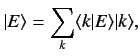(603)

where the summation is from to . Substituting the above equation into Equation (602), and right-multiplying by $\langle m\vert$ , we obtain

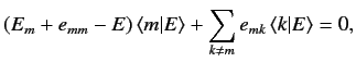$\displaystyle (E_m + e_{mm} - E)\, \langle m\vert E\rangle + \sum_{k\neq m} e_{mk}\, \langle k\vert E\rangle = 0,$

(604)

where

$\displaystyle e_{mk} = \langle m \vert\,H_1\,\vert k\rangle.$

(605)

Let us now develop our perturbation expansion. We assume that

$\displaystyle \frac{\vert e_{mk}\vert}{E_m - E_k} \sim O(\epsilon),$

(606)

for all $m\neq k$ , where $\epsilon\ll 1$ is our expansion parameter. We also assume that

$\displaystyle \frac{\vert e_{mm}\vert}{E_m} \sim O(\epsilon),$

(607)

for all . Let us search for a modified version of the th unperturbed energy eigenstate, for which

$\displaystyle E= E_n + O(\epsilon),$

(608)

and

$\displaystyle \langle n\vert E\rangle$	$\displaystyle =$	$\displaystyle 1,$	(609)
$\displaystyle \langle m\vert E\rangle$	$\displaystyle \sim$	$\displaystyle O(\epsilon),$	(610)

for $m\neq n$ . Suppose that we write out Equation (604) for $m\neq n$ , neglecting terms that are $O(\epsilon^2)$ according to our expansion scheme. We find that

$\displaystyle (E_m - E_n) \,\langle m \vert E \rangle + e_{mn} \simeq 0,$

(611)

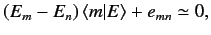
giving

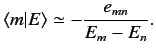$\displaystyle \langle m\vert E\rangle \simeq -\frac{e_{mn}}{E_m - E_n}.$

(612)

Substituting the above expression into Equation (604), evaluated for , and neglecting $O(\epsilon^3)$ terms, we obtain

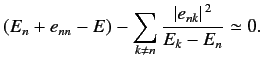$\displaystyle (E_n + e_{nn} - E) - \sum_{k\neq n} \frac{\vert e_{nk}\vert^{\,2}} {E_k-E_n} \simeq 0.$

(613)

Thus, the modified th energy eigenstate possesses an eigenvalue

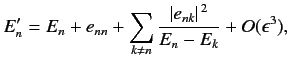$\displaystyle E_n' = E_n + e_{nn} + \sum_{k\neq n} \frac{\vert e_{nk}\vert^{\,2}} {E_n-E_k} + O(\epsilon^3),$

(614)

and a eigenket

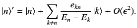$\displaystyle \vert n\rangle' = \vert n\rangle +\sum_{k\neq n}\frac{e_{kn}}{E_n - E_k}\,\vert k\rangle + O(\epsilon^2).$

(615)

Note that

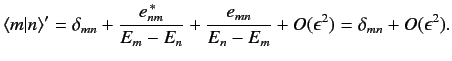$\displaystyle \langle m\vert n\rangle' = \delta_{mn} + \frac{e_{nm}^{\,\ast}}{E_m-E_n} + \frac{e_{mn}} {E_n-E_m} + O(\epsilon^2) = \delta_{mn} + O(\epsilon^2).$

(616)

Thus, the modified eigenkets remain orthogonal and properly normalized to $O(\epsilon^2)$ .

Next: Quadratic Stark Effect Up: Time-Independent Perturbation Theory Previous: Two-State System

Richard Fitzpatrick 2013-04-08