Heisenberg Equation of Motion

We have seen that in the Schrödinger scheme the dynamical variables of the system remain fixed during a period of undisturbed motion, whereas the state kets evolve according to Equation (229). However, this is not the only way in which to represent the time evolution of the system.

Suppose that a general state ket $A$ is subject to the transformation

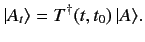$$\vert A_t \rangle = T^{\dag }(t, t_0)\, \vert A\rangle.$$ (235)

This is a time-dependent transformation, because the operator $T(t, t_0)$ obviously depends on time. The subscript $t$ is used to remind us that the transformation is time-dependent. The time evolution of the transformed state ket is given by

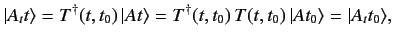$$\vert A_t t\rangle = T^{\dag } (t, t_0)\,\vert At\rangle = T^{\dag } (t, t_0)\,T (t, t_0)\, \vert At_0\rangle = \vert A_t t_0\rangle,$$ (236)

where use has been made of Equations (222), (224), and the fact that $T(t_0, t_0)=1$ . Clearly, the transformed state ket does not evolve in time. Thus, the transformation (235) has the effect of bringing all kets representing states of undisturbed motion of the system to rest.

The transformation must also be applied to bras. The dual of Equation (235) yields

$$\langle A_t\vert =\langle A\vert \,T.$$ (237)

The transformation rule for a general observable $v$ is obtained from the requirement that the expectation value $\langle A\vert\,v\,\vert A\rangle$ should remain invariant. It is easily seen that

$$v_t = T^{\dag } \,v \,T.$$ (238)

Thus, a dynamical variable, which corresponds to a fixed linear operator in Schrödinger's scheme, corresponds to a moving linear operator in this new scheme. It is clear that the transformation (235) leads us to a scenario in which the state of the system is represented by a fixed vector, and the dynamical variables are represented by moving linear operators. This is termed the Heisenberg picture, as opposed to the Schrödinger picture, which is outlined in Section 3.1.

Consider a dynamical variable $v$ corresponding to a fixed linear operator in the Schrödinger picture. According to Equation (238), we can write

$$T \,v_t = v\, T.$$ (239)

Differentiation with respect to time yields

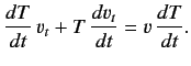$$\frac{d T}{dt} \,v_t + T \,\frac{dv_t}{dt} = v\, \frac{dT}{dt}.$$ (240)

With the help of Equation (233), this reduces to

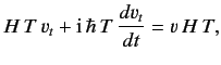$$H\,T\, v_t +{\rm i}\,\hbar\, T\,\frac{d v_t}{dt} = v\, H\,T,$$ (241)

or

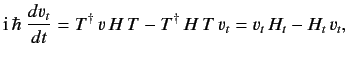$${\rm i}\,\hbar\ \frac{d v_t}{dt} = T^{\dag } \,v \,H\,T - T^{\dag } \,H\,T \,v_t = v_t\, H_t - H_t\, v_t,$$ (242)

where

$$H_t = T^{\dag }\, H\, T.$$ (243)

Equation (242) can be written

$${\rm i}\,\hbar\ \frac{d v_t}{dt} = [v_t, H_t].$$ (244)

Equation (244) shows how the dynamical variables of the system evolve in the Heisenberg picture. It is denoted the Heisenberg equation of motion. Note that the time-varying dynamical variables in the Heisenberg picture are usually called Heisenberg dynamical variables to distinguish them from Schrödinger dynamical variables (i.e., the corresponding variables in the Schrödinger picture), which do not evolve in time.

According to Equation (113), the Heisenberg equation of motion can be written

$$\frac{dv_t}{dt} = [v_t, H_t]_{qm},$$ (245)

where $[\cdots]_{qm}$ denotes the quantum Poisson bracket. Let us compare this equation with the classical time evolution equation for a general dynamical variable $v$ , which can be written in the form [see Equation (98)]

$$\frac{dv}{dt} = [v,H]_{cl}.$$ (246)

Here, $[\cdots]_{cl}$ is the classical Poisson bracket, and $H$ denotes the classical Hamiltonian. The strong resemblance between Equations (245) and (246) provides us with further justification for our identification of the linear operator $H$ with the energy of the system in quantum mechanics.

Note that if the Hamiltonian does not explicitly depend on time (i.e., the system is not subject to some time-dependent external force) then Equation (234) yields

$$T(t, t_0) = \exp\left[-{\rm i}\, H\,(t-t_0)/\hbar \right].$$ (247)

This operator manifestly commutes with $H$ , so

$$H_t = T^{\dag }\, H \,T = H.$$ (248)

Furthermore, Equation (244) gives

$${\rm i}\,\hbar \,\frac{dH}{dt} = [H, H] = 0.$$ (249)

Thus, if the energy of the system has no explicit time-dependence then it is represented by the same non-time-varying operator $H$ in both the Schrödinger and Heisenberg pictures.

Suppose that $v$ is an observable that commutes with the Hamiltonian (and, hence, with the time evolution operator $T$ ). It follows from Equation (238) that $v_t= v$ . Heisenberg's equation of motion yields

$${\rm i}\,\hbar \,\frac{d v}{dt} = [v, H] = 0.$$ (250)

Thus, any observable that commutes with the Hamiltonian is a constant of the motion (hence, it is represented by the same fixed operator in both the Schrödinger and Heisenberg pictures). Only those observables that do not commute with the Hamiltonian evolve in time in the Heisenberg picture.