Continuous Spectra

Up to now, we have studiously avoided dealing with observables possessing eigenvalues that lie in a continuous range, rather than having discrete values. The reason for this is that continuous eigenvalues imply a ket space of nondenumerably infinite dimension. Unfortunately, continuous eigenvalues are unavoidable in quantum mechanics. In fact, the most important observables of all--namely position and momentum--generally have continuous eigenvalues. Fortunately, many of the results that we obtained previously for a finite-dimensional ket space with discrete eigenvalues can be generalized to ket spaces of nondenumerably infinite dimensions.

Suppose that $\xi$ is an observable with continuous eigenvalues. We can still write the eigenvalue equation as

$$\xi \,\vert\xi'\rangle =\xi'\, \vert\xi'\rangle.$$ (84)

But, $\xi'$ can now take a continuous range of values. Let us assume, for the sake of simplicity, that $\xi'$ can take any value. The orthogonality condition (50) generalizes to

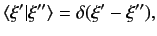$$\langle \xi'\vert\xi''\rangle = \delta(\xi'-\xi''),$$ (85)

where $\delta(x)$ denotes the famous Dirac delta function, and satisfies

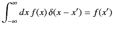$$\int_{-\infty}^\infty dx\,f(x)\,\delta(x-x') =f(x')$$ (86)

for any function, $f(x)$ , that is well-behaved at $x=x'$ . Note that there are clearly a nondenumerably infinite number of mutually orthogonal eigenstates of $\xi$ . Hence, the dimensionality of ket space is nondenumerably infinite. Furthermore, eigenstates corresponding to a continuous range of eigenvalues cannot be normalized such that they have unit norms. In fact, these eigenstates have infinite norms: i.e., they are infinitely long. This is the major difference between eigenstates in a finite-dimensional and an infinite-dimensional ket space. The extremely useful relation (54) generalizes to

$$\int d\xi' \,\vert\xi'\rangle\langle \xi'\vert = 1.$$ (87)

Note that a summation over discrete eigenvalues goes over into an integral over a continuous range of eigenvalues. The eigenstates $\vert\xi'\rangle$ must form a complete set if $\xi$ is to be an observable. It follows that any general ket can be expanded in terms of the $\vert\xi'\rangle$ . In fact, the expansions (51)-(53) generalize to

$$\vert A\rangle = \int d\xi'\,\vert\xi'\rangle\langle \xi'\vert A\rangle,$$ (88)

$$\langle A\vert = \int d\xi'\,\langle A\vert\xi'\rangle \langle \xi'\vert,$$ (89)

$$\langle A\vert A\rangle = \int d\xi'\,\langle A\vert\xi'\rangle\langle \xi'\vert A\rangle = \int d\xi' \,\vert\langle A\vert\xi'\rangle\vert^{\,2}.$$ (90)

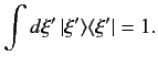
These results also follow simply from Equation (87). We have seen that it is not possible to normalize the eigenstates $\vert\xi'\rangle$ such that they have unit norms. Fortunately, this convenient normalization is still possible for a general state vector. In fact, according to Equation (90), the normalization condition can be written

$$\langle A\vert A\rangle =\int d\xi' \,\vert\langle A\vert\xi'\rangle\vert^{\,2} = 1.$$ (91)

We have now studied observables whose eigenvalues take a discrete number of values, as well as those whose eigenvalues take a continuous range of values. There are a number of other cases we could look at. For instance, observables whose eigenvalues can take a (finite) continuous range of values, plus a set of discrete values. Such cases can be dealt with using a fairly straightforward generalization of the previous analysis (see Dirac, Chapters II and III).